Latent Growth Models
In this tutorial, we are going to use lavaan for latent
growth models.
Load the pacakges
library(lavaan)
library(semPlot)
Example: Linear LGM (1)
The data for this example are from 1000 school girls, whose math self-concept has been measured repeatedly at 9th, 10th, 11th, and 12th grade.
Read the data
lower <- '
2.041
1.392  1.901
1.366  1.352  1.665
1.249  1.303  1.348  1.599
'

smeans <- c(3.297, 3.614, 4.042, 4.375)
covmat <- getCov(lower)
rownames(covmat) <- colnames(covmat) <- paste0('mathsc', 9:12)
Fit the model to the data
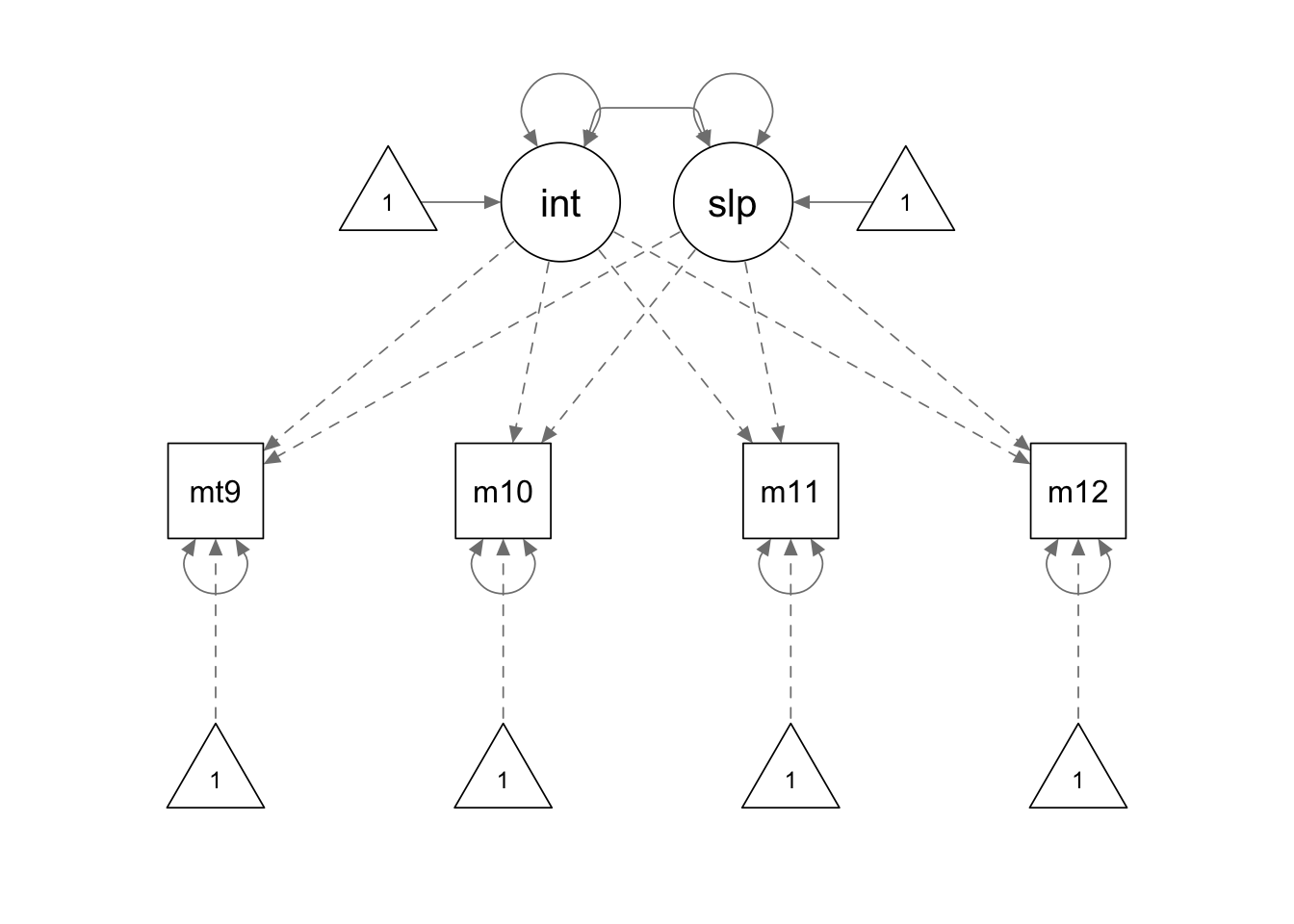
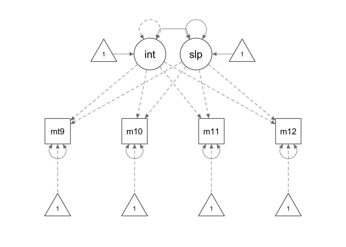
To fit a linear latent growth model, we can use the special function
growth() in lavaan package. When we write the
model syntax, we only need to define the latent intercept and latent
slope; the loadings have to be fixed manually based on your time
scale.
The growth() function is a special case of the
sem() function that we have been using. But
growth() makes things easier when you deal with a simple
LGM. Using this function, you do not need to manually specify the mean
structure as it is automatically assumed. You do not need to manually
fix the observed intercepts to zero, which is taken care of by default.
The means of the latent variables are freely estimated by default.
growth.model1 <- '
interc =~ 1*mathsc9 + 1*mathsc10 + 1*mathsc11 + 1*mathsc12
slope =~ 0*mathsc9 + 1*mathsc10 + 2*mathsc11 + 3*mathsc12
'

growth.fit1 <- growth(growth.model1, sample.cov = covmat, sample.mean = smeans, sample.nobs = 1000)
summary(growth.fit1, fit.measures = T, standardized = T)
## lavaan 0.6.15 ended normally after 31 iterations
##
## Estimator ML
## Optimization method NLMINB
## Number of model parameters 9
##
## Number of observations 1000
##
## Model Test User Model:
##
## Test statistic 8.256
## Degrees of freedom 5
## P-value (Chi-square) 0.143
##
## Model Test Baseline Model:
##
## Test statistic 3045.699
## Degrees of freedom 6
## P-value 0.000
##
## User Model versus Baseline Model:
##
## Comparative Fit Index (CFI) 0.999
## Tucker-Lewis Index (TLI) 0.999
##
## Loglikelihood and Information Criteria:
##
## Loglikelihood user model (H0) -5322.543
## Loglikelihood unrestricted model (H1) -5318.415
##
## Akaike (AIC) 10663.087
## Bayesian (BIC) 10707.256
## Sample-size adjusted Bayesian (SABIC) 10678.672
##
## Root Mean Square Error of Approximation:
##
## RMSEA 0.026
## 90 Percent confidence interval - lower 0.000
## 90 Percent confidence interval - upper 0.055
## P-value H_0: RMSEA <= 0.050 0.903
## P-value H_0: RMSEA >= 0.080 0.001
##
## Standardized Root Mean Square Residual:
##
## SRMR 0.012
##
## Parameter Estimates:
##
## Standard errors Standard
## Information Expected
## Information saturated (h1) model Structured
##
## Latent Variables:
## Estimate Std.Err z-value P(>|z|) Std.lv Std.all
## interc =~
## mathsc9 1.000 1.219 0.851
## mathsc10 1.000 1.219 0.881
## mathsc11 1.000 1.219 0.953
## mathsc12 1.000 1.219 0.960
## slope =~
## mathsc9 0.000 0.000 0.000
## mathsc10 1.000 0.190 0.137
## mathsc11 2.000 0.380 0.297
## mathsc12 3.000 0.569 0.449
##
## Covariances:
## Estimate Std.Err z-value P(>|z|) Std.lv Std.all
## interc ~~
## slope -0.072 0.018 -3.944 0.000 -0.311 -0.311
##
## Intercepts:
## Estimate Std.Err z-value P(>|z|) Std.lv Std.all
## .mathsc9 0.000 0.000 0.000
## .mathsc10 0.000 0.000 0.000
## .mathsc11 0.000 0.000 0.000
## .mathsc12 0.000 0.000 0.000
## interc 3.286 0.043 76.434 0.000 2.697 2.697
## slope 0.365 0.011 34.516 0.000 1.926 1.926
##
## Variances:
## Estimate Std.Err z-value P(>|z|) Std.lv Std.all
## .mathsc9 0.565 0.044 12.776 0.000 0.565 0.275
## .mathsc10 0.535 0.030 17.891 0.000 0.535 0.280
## .mathsc11 0.294 0.020 14.766 0.000 0.294 0.180
## .mathsc12 0.233 0.027 8.523 0.000 0.233 0.144
## interc 1.485 0.085 17.488 0.000 1.000 1.000
## slope 0.036 0.007 4.963 0.000 1.000 1.000Same Model with Homoscedastic Error Variance
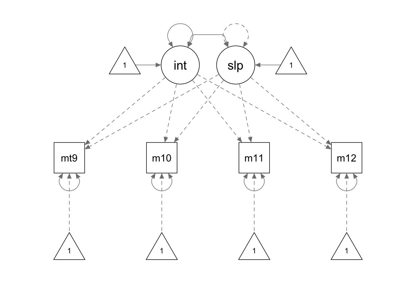
hs.model <- '
interc =~ 1*mathsc9 + 1*mathsc10 + 1*mathsc11 + 1*mathsc12
slope =~ 0*mathsc9 + 1*mathsc10 + 2*mathsc11 + 3*mathsc12

# constrain the error variance
mathsc9 ~~ a*mathsc9
mathsc10 ~~ a*mathsc10
mathsc11 ~~ a*mathsc11
mathsc12 ~~ a*mathsc12
'

hs.fit <- growth(hs.model, sample.cov = covmat, sample.mean = smeans, sample.nobs = 1000)

summary(hs.fit, fit.measures = T, standardized = F)
## lavaan 0.6.15 ended normally after 28 iterations
##
## Estimator ML
## Optimization method NLMINB
## Number of model parameters 9
## Number of equality constraints 3
##
## Number of observations 1000
##
## Model Test User Model:
##
## Test statistic 134.023
## Degrees of freedom 8
## P-value (Chi-square) 0.000
##
## Model Test Baseline Model:
##
## Test statistic 3045.699
## Degrees of freedom 6
## P-value 0.000
##
## User Model versus Baseline Model:
##
## Comparative Fit Index (CFI) 0.959
## Tucker-Lewis Index (TLI) 0.969
##
## Loglikelihood and Information Criteria:
##
## Loglikelihood user model (H0) -5385.427
## Loglikelihood unrestricted model (H1) -5318.415
##
## Akaike (AIC) 10782.853
## Bayesian (BIC) 10812.300
## Sample-size adjusted Bayesian (SABIC) 10793.244
##
## Root Mean Square Error of Approximation:
##
## RMSEA 0.126
## 90 Percent confidence interval - lower 0.107
## 90 Percent confidence interval - upper 0.145
## P-value H_0: RMSEA <= 0.050 0.000
## P-value H_0: RMSEA >= 0.080 1.000
##
## Standardized Root Mean Square Residual:
##
## SRMR 0.030
##
## Parameter Estimates:
##
## Standard errors Standard
## Information Expected
## Information saturated (h1) model Structured
##
## Latent Variables:
## Estimate Std.Err z-value P(>|z|)
## interc =~
## mathsc9 1.000
## mathsc10 1.000
## mathsc11 1.000
## mathsc12 1.000
## slope =~
## mathsc9 0.000
## mathsc10 1.000
## mathsc11 2.000
## mathsc12 3.000
##
## Covariances:
## Estimate Std.Err z-value P(>|z|)
## interc ~~
## slope -0.096 0.017 -5.794 0.000
##
## Intercepts:
## Estimate Std.Err z-value P(>|z|)
## .mathsc9 0.000
## .mathsc10 0.000
## .mathsc11 0.000
## .mathsc12 0.000
## interc 3.283 0.043 76.325 0.000
## slope 0.366 0.011 34.068 0.000
##
## Variances:
## Estimate Std.Err z-value P(>|z|)
## .mathsc9 (a) 0.411 0.013 31.623 0.000
## .mathsc10 (a) 0.411 0.013 31.623 0.000
## .mathsc11 (a) 0.411 0.013 31.623 0.000
## .mathsc12 (a) 0.411 0.013 31.623 0.000
## interc 1.562 0.083 18.767 0.000
## slope 0.033 0.006 5.754 0.000Example: Linear LGM (2)
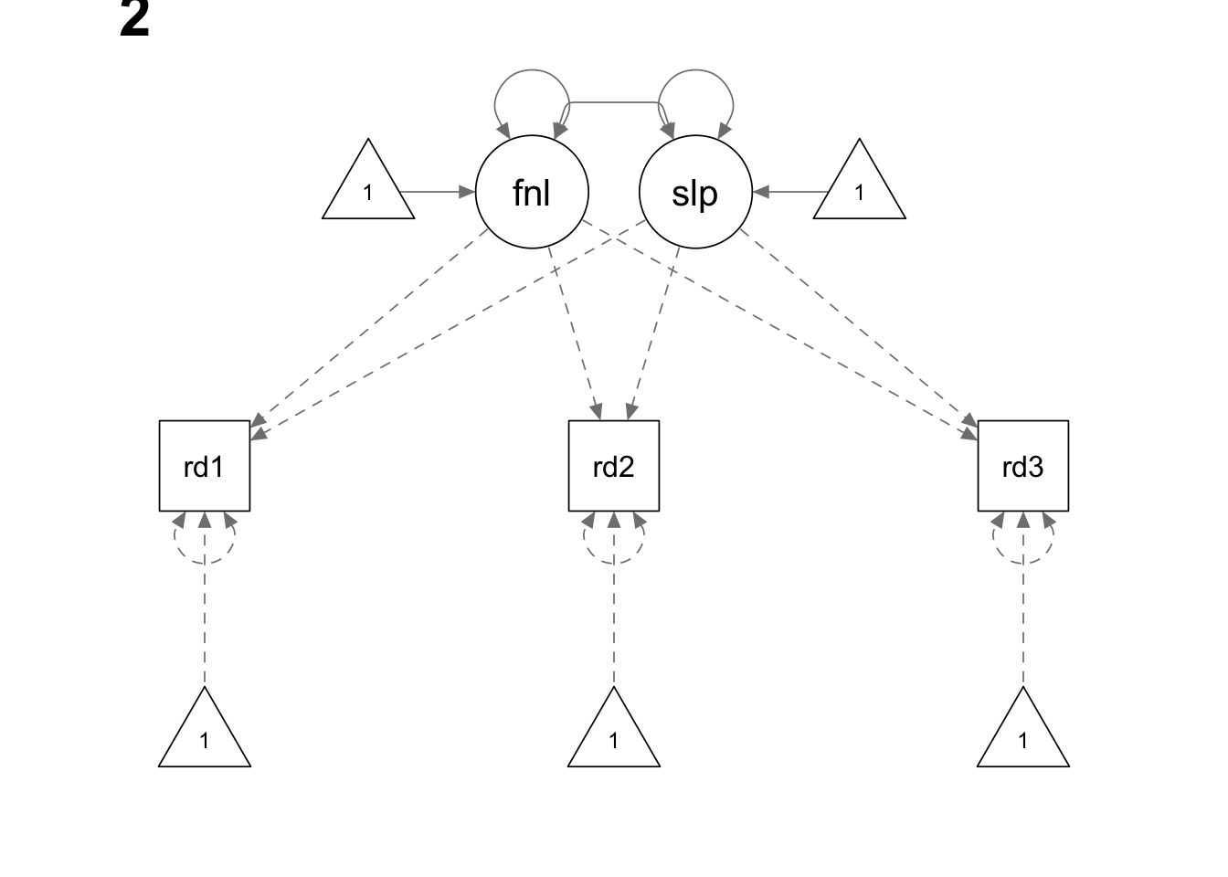
The data for this example are from 324 non-native English speakers, whose reading ability has been measured at three equally spaced time points (1 month apart).
Read the data
lower <- '
42.92
32.06 39.35
29.67 28.80 37.43
'
smeans <- c(17.08, 18.40, 19.23)

covmat <- getCov(lower)
colnames(covmat) <- c("read1","read2","read3")
rownames(covmat) <- colnames(covmat)
Fit the model to the data
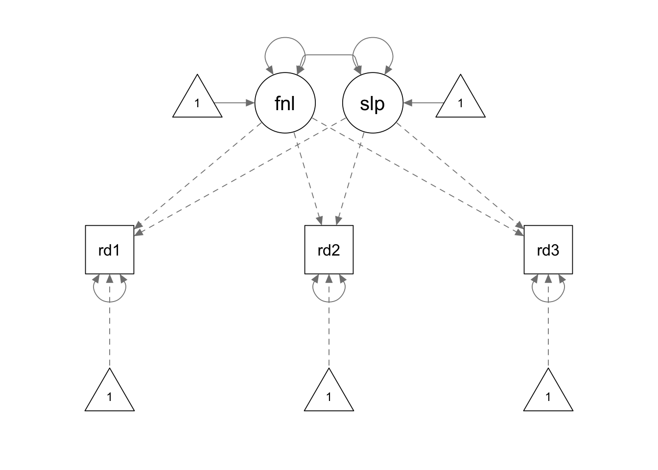
Note that in this example we use the last measurement point as the reference point. Therefore, its loading on the latent slope is fixed to zero. The first measurement has a loading of -2 and the second measurement has a loading of -1. Accordingly, the interpretation of the “intercept” latent factor is no longer the level of reading ability at the initial measurement; instead, it reflects the level of reading ability at the last measurement.
Heterogeneous error structure
growth.model2.he <- '
final =~ 1*read1 + 1*read2 + 1*read3
slope =~ (-2)*read1 + (-1)*read2 + 0*read3

read1 ~~ read1
read2 ~~ read2
read3 ~~ read3
'

growth.fit2.he <- growth(growth.model2.he, sample.cov = covmat, sample.mean = smeans, sample.nobs = 324)
summary(growth.fit2.he, fit.measures = T)
## lavaan 0.6.15 ended normally after 71 iterations
##
## Estimator ML
## Optimization method NLMINB
## Number of model parameters 8
##
## Number of observations 324
##
## Model Test User Model:
##
## Test statistic 1.451
## Degrees of freedom 1
## P-value (Chi-square) 0.228
##
## Model Test Baseline Model:
##
## Test statistic 621.168
## Degrees of freedom 3
## P-value 0.000
##
## User Model versus Baseline Model:
##
## Comparative Fit Index (CFI) 0.999
## Tucker-Lewis Index (TLI) 0.998
##
## Loglikelihood and Information Criteria:
##
## Loglikelihood user model (H0) -2858.645
## Loglikelihood unrestricted model (H1) -2857.920
##
## Akaike (AIC) 5733.291
## Bayesian (BIC) 5763.537
## Sample-size adjusted Bayesian (SABIC) 5738.161
##
## Root Mean Square Error of Approximation:
##
## RMSEA 0.037
## 90 Percent confidence interval - lower 0.000
## 90 Percent confidence interval - upper 0.158
## P-value H_0: RMSEA <= 0.050 0.398
## P-value H_0: RMSEA >= 0.080 0.403
##
## Standardized Root Mean Square Residual:
##
## SRMR 0.011
##
## Parameter Estimates:
##
## Standard errors Standard
## Information Expected
## Information saturated (h1) model Structured
##
## Latent Variables:
## Estimate Std.Err z-value P(>|z|)
## final =~
## read1 1.000
## read2 1.000
## read3 1.000
## slope =~
## read1 -2.000
## read2 -1.000
## read3 0.000
##
## Covariances:
## Estimate Std.Err z-value P(>|z|)
## final ~~
## slope -0.888 1.447 -0.614 0.539
##
## Intercepts:
## Estimate Std.Err z-value P(>|z|)
## .read1 0.000
## .read2 0.000
## .read3 0.000
## final 19.317 0.332 58.244 0.000
## slope 1.080 0.127 8.497 0.000
##
## Variances:
## Estimate Std.Err z-value P(>|z|)
## .read1 8.482 2.705 3.135 0.002
## .read2 8.932 1.369 6.526 0.000
## .read3 9.513 2.543 3.741 0.000
## final 27.809 3.268 8.508 0.000
## slope 0.738 1.296 0.569 0.569Same model: With homogeneous error structure
growth.model2 <- '

final =~ 1*read1 + 1*read2 + 1*read3
slope =~ (-2)*read1 + (-1)*read2 + 0*read3

# fix the error variances
read1 ~~ a*read1
read2 ~~ a*read2
read3 ~~ a*read3
'

growth.fit2 <- growth(growth.model2, sample.cov = covmat, sample.mean = smeans, sample.nobs = 324)
summary(growth.fit2, fit.measures = T)
## lavaan 0.6.15 ended normally after 60 iterations
##
## Estimator ML
## Optimization method NLMINB
## Number of model parameters 8
## Number of equality constraints 2
##
## Number of observations 324
##
## Model Test User Model:
##
## Test statistic 1.763
## Degrees of freedom 3
## P-value (Chi-square) 0.623
##
## Model Test Baseline Model:
##
## Test statistic 621.168
## Degrees of freedom 3
## P-value 0.000
##
## User Model versus Baseline Model:
##
## Comparative Fit Index (CFI) 1.000
## Tucker-Lewis Index (TLI) 1.002
##
## Loglikelihood and Information Criteria:
##
## Loglikelihood user model (H0) -2858.801
## Loglikelihood unrestricted model (H1) -2857.920
##
## Akaike (AIC) 5729.602
## Bayesian (BIC) 5752.287
## Sample-size adjusted Bayesian (SABIC) 5733.255
##
## Root Mean Square Error of Approximation:
##
## RMSEA 0.000
## 90 Percent confidence interval - lower 0.000
## 90 Percent confidence interval - upper 0.076
## P-value H_0: RMSEA <= 0.050 0.839
## P-value H_0: RMSEA >= 0.080 0.041
##
## Standardized Root Mean Square Residual:
##
## SRMR 0.011
##
## Parameter Estimates:
##
## Standard errors Standard
## Information Expected
## Information saturated (h1) model Structured
##
## Latent Variables:
## Estimate Std.Err z-value P(>|z|)
## final =~
## read1 1.000
## read2 1.000
## read3 1.000
## slope =~
## read1 -2.000
## read2 -1.000
## read3 0.000
##
## Covariances:
## Estimate Std.Err z-value P(>|z|)
## final ~~
## slope -0.695 0.863 -0.805 0.421
##
## Intercepts:
## Estimate Std.Err z-value P(>|z|)
## .read1 0.000
## .read2 0.000
## .read3 0.000
## final 19.312 0.332 58.224 0.000
## slope 1.075 0.127 8.456 0.000
##
## Variances:
## Estimate Std.Err z-value P(>|z|)
## .read1 (a) 8.954 0.703 12.728 0.000
## .read2 (a) 8.954 0.703 12.728 0.000
## .read3 (a) 8.954 0.703 12.728 0.000
## final 28.182 2.861 9.850 0.000
## slope 0.759 0.541 1.403 0.161Example: Linear LGM (3)
Read the data
lower <- '
1.000
0.725 1.000
0.595 0.705 1.000
0.566 0.624 0.706 1.000
'

smeans <- c(1.338, 1.591, 2.019, 2.364)
sds <- c(1.260, 1.334, 1.440, 1.376)
covmat <- diag(sds) %*% getCov(lower) %*% diag(sds)
rownames(covmat) <- colnames(covmat) <- paste0('alc', c(12, 14, 16, 18))
Fit the model to the data
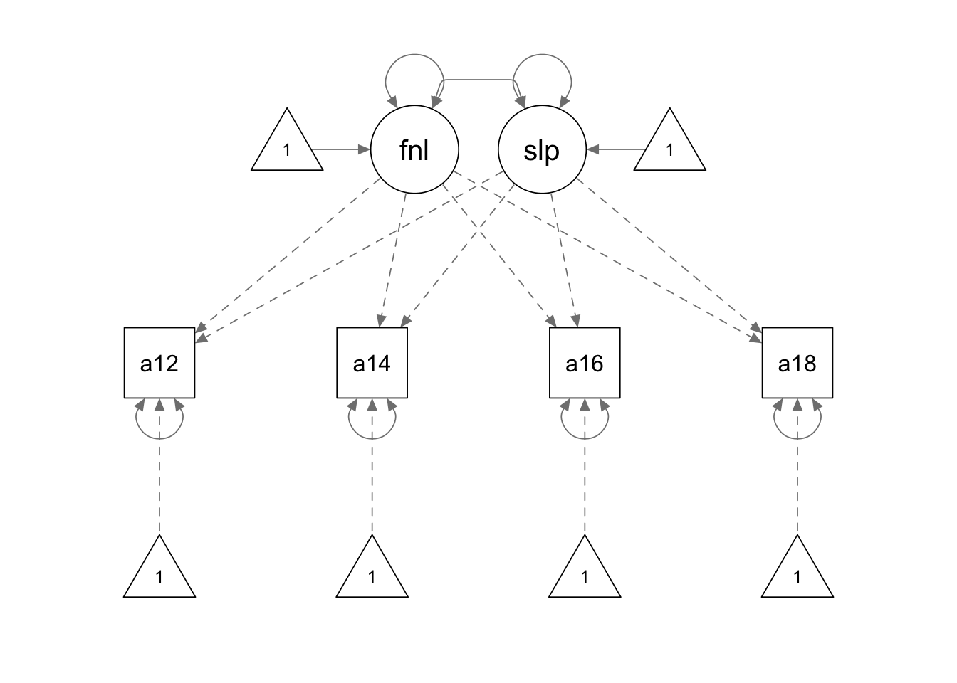
growth.model3 <- '

final =~ 1*alc12 + 1*alc14 + 1*alc16 + 1*alc18
slope =~ -6*alc12 + -4*alc14 + -2*alc16 + 0*alc18

'

growth.fit3 <- growth(growth.model3, sample.cov = covmat, sample.mean = smeans, sample.nobs = 357)

summary(growth.fit3, fit.measures = T)
## lavaan 0.6.15 ended normally after 33 iterations
##
## Estimator ML
## Optimization method NLMINB
## Number of model parameters 9
##
## Number of observations 357
##
## Model Test User Model:
##
## Test statistic 20.799
## Degrees of freedom 5
## P-value (Chi-square) 0.001
##
## Model Test Baseline Model:
##
## Test statistic 799.900
## Degrees of freedom 6
## P-value 0.000
##
## User Model versus Baseline Model:
##
## Comparative Fit Index (CFI) 0.980
## Tucker-Lewis Index (TLI) 0.976
##
## Loglikelihood and Information Criteria:
##
## Loglikelihood user model (H0) -2064.204
## Loglikelihood unrestricted model (H1) -2053.804
##
## Akaike (AIC) 4146.408
## Bayesian (BIC) 4181.308
## Sample-size adjusted Bayesian (SABIC) 4152.756
##
## Root Mean Square Error of Approximation:
##
## RMSEA 0.094
## 90 Percent confidence interval - lower 0.055
## 90 Percent confidence interval - upper 0.138
## P-value H_0: RMSEA <= 0.050 0.035
## P-value H_0: RMSEA >= 0.080 0.748
##
## Standardized Root Mean Square Residual:
##
## SRMR 0.038
##
## Parameter Estimates:
##
## Standard errors Standard
## Information Expected
## Information saturated (h1) model Structured
##
## Latent Variables:
## Estimate Std.Err z-value P(>|z|)
## final =~
## alc12 1.000
## alc14 1.000
## alc16 1.000
## alc18 1.000
## slope =~
## alc12 -6.000
## alc14 -4.000
## alc16 -2.000
## alc18 0.000
##
## Covariances:
## Estimate Std.Err z-value P(>|z|)
## final ~~
## slope 0.084 0.020 4.293 0.000
##
## Intercepts:
## Estimate Std.Err z-value P(>|z|)
## .alc12 0.000
## .alc14 0.000
## .alc16 0.000
## .alc18 0.000
## final 2.351 0.072 32.579 0.000
## slope 0.174 0.011 16.003 0.000
##
## Variances:
## Estimate Std.Err z-value P(>|z|)
## .alc12 0.359 0.069 5.191 0.000
## .alc14 0.510 0.051 9.962 0.000
## .alc16 0.673 0.064 10.588 0.000
## .alc18 0.444 0.082 5.395 0.000
## final 1.524 0.147 10.378 0.000
## slope 0.021 0.004 5.011 0.000modindices(growth.fit3, minimum.value = 3.89, sort. = T) #modification indices## lhs op rhs mi epc sepc.lv sepc.all sepc.nox
## 25 alc14 ~~ alc16 15.516 0.193 0.193 0.330 0.330
## 26 alc14 ~~ alc18 9.151 -0.148 -0.148 -0.310 -0.310
## 23 alc12 ~~ alc16 8.519 -0.137 -0.137 -0.279 -0.279
## 6 slope =~ alc14 5.575 -0.553 -0.081 -0.062 -0.062
## 24 alc12 ~~ alc18 5.549 0.157 0.157 0.395 0.395
## 17 alc14 ~1 4.081 -0.088 -0.088 -0.068 -0.068Same model: With structured errors
se.model <- '

final =~ 1*alc12 + 1*alc14 + 1*alc16 + 1*alc18
slope =~ -6*alc12 + -4*alc14 + -2*alc16 + 0*alc18

final ~ 1
slope ~ 1

alc12 ~ 0*1
alc14 ~ 0*1
alc16 ~ 0*1
alc18 ~ 0*1

# explicitly model the errors

E12 =~ alc12
E14 =~ alc14
E16 =~ alc16
E18 =~ alc18

E14 ~ E12
E16 ~ E14
E18 ~ E16

# model constraints

alc12 ~~ 0*alc12
alc14 ~~ 0*alc14
alc16 ~~ 0*alc16
alc18 ~~ 0*alc18

E12 ~~ 0*final + 0*slope

E12 ~ 0*1
E14 ~ 0*1
E16 ~ 0*1
E18 ~ 0*1

'
se.fit <- sem(se.model, sample.cov = covmat, sample.mean = smeans, sample.nobs = 357)

summary(se.fit, fit.measures = T)
## lavaan 0.6.15 ended normally after 50 iterations
##
## Estimator ML
## Optimization method NLMINB
## Number of model parameters 12
##
## Number of observations 357
##
## Model Test User Model:
##
## Test statistic 4.332
## Degrees of freedom 2
## P-value (Chi-square) 0.115
##
## Model Test Baseline Model:
##
## Test statistic 799.900
## Degrees of freedom 6
## P-value 0.000
##
## User Model versus Baseline Model:
##
## Comparative Fit Index (CFI) 0.997
## Tucker-Lewis Index (TLI) 0.991
##
## Loglikelihood and Information Criteria:
##
## Loglikelihood user model (H0) -2055.970
## Loglikelihood unrestricted model (H1) -2053.804
##
## Akaike (AIC) 4135.940
## Bayesian (BIC) 4182.473
## Sample-size adjusted Bayesian (SABIC) 4144.404
##
## Root Mean Square Error of Approximation:
##
## RMSEA 0.057
## 90 Percent confidence interval - lower 0.000
## 90 Percent confidence interval - upper 0.132
## P-value H_0: RMSEA <= 0.050 0.335
## P-value H_0: RMSEA >= 0.080 0.381
##
## Standardized Root Mean Square Residual:
##
## SRMR 0.015
##
## Parameter Estimates:
##
## Standard errors Standard
## Information Expected
## Information saturated (h1) model Structured
##
## Latent Variables:
## Estimate Std.Err z-value P(>|z|)
## final =~
## alc12 1.000
## alc14 1.000
## alc16 1.000
## alc18 1.000
## slope =~
## alc12 -6.000
## alc14 -4.000
## alc16 -2.000
## alc18 0.000
## E12 =~
## alc12 1.000
## E14 =~
## alc14 1.000
## E16 =~
## alc16 1.000
## E18 =~
## alc18 1.000
##
## Regressions:
## Estimate Std.Err z-value P(>|z|)
## E14 ~
## E12 0.283 0.512 0.552 0.581
## E16 ~
## E14 0.378 0.112 3.360 0.001
## E18 ~
## E16 0.205 0.230 0.889 0.374
##
## Covariances:
## Estimate Std.Err z-value P(>|z|)
## final ~~
## E12 0.000
## slope ~~
## E12 0.000
## final ~~
## slope 0.059 0.061 0.978 0.328
##
## Intercepts:
## Estimate Std.Err z-value P(>|z|)
## final 2.353 0.072 32.768 0.000
## slope 0.172 0.011 15.937 0.000
## .alc12 0.000
## .alc14 0.000
## .alc16 0.000
## .alc18 0.000
## E12 0.000
## .E14 0.000
## .E16 0.000
## .E18 0.000
##
## Variances:
## Estimate Std.Err z-value P(>|z|)
## .alc12 0.000
## .alc14 0.000
## .alc16 0.000
## .alc18 0.000
## final 1.326 0.370 3.587 0.000
## slope 0.015 0.017 0.904 0.366
## E12 0.430 0.541 0.794 0.427
## .E14 0.655 0.107 6.128 0.000
## .E16 0.821 0.147 5.592 0.000
## .E18 0.524 0.268 1.954 0.051Example: LGM with Linear Stability
lower <- '
2.041
1.392  1.901
1.366  1.352  1.665
1.249  1.303  1.348  1.599
'

smeans <- c(3.297,  3.614,  4.042,  4.375)

covmat <- getCov(lower)
rownames(covmat) <- colnames(covmat) <- paste0('mathsc', 9:12)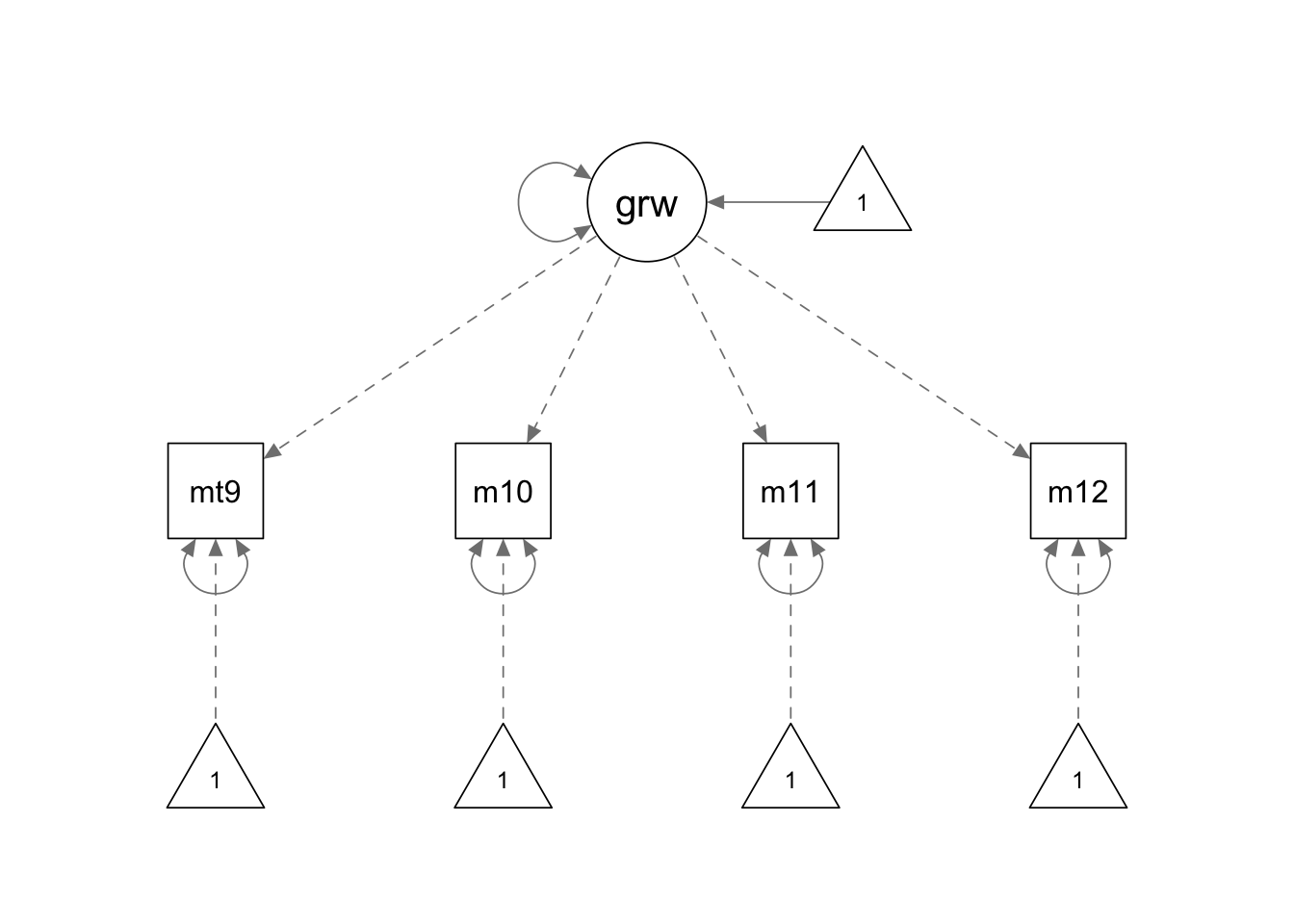
ls.model <- '

growth =~ 1*mathsc9+2*mathsc10+3*mathsc11+4*mathsc12
growth ~ 1
'

ls.fit <- growth(ls.model, sample.cov = covmat, sample.mean = smeans, sample.nobs = 1000)


summary(ls.fit, fit.measures = T, standardized = F)
## lavaan 0.6.15 ended normally after 35 iterations
##
## Estimator ML
## Optimization method NLMINB
## Number of model parameters 6
##
## Number of observations 1000
##
## Model Test User Model:
##
## Test statistic 4065.273
## Degrees of freedom 8
## P-value (Chi-square) 0.000
##
## Model Test Baseline Model:
##
## Test statistic 3045.699
## Degrees of freedom 6
## P-value 0.000
##
## User Model versus Baseline Model:
##
## Comparative Fit Index (CFI) 0.000
## Tucker-Lewis Index (TLI) -0.001
##
## Loglikelihood and Information Criteria:
##
## Loglikelihood user model (H0) -7351.052
## Loglikelihood unrestricted model (H1) -5318.415
##
## Akaike (AIC) 14714.103
## Bayesian (BIC) 14743.550
## Sample-size adjusted Bayesian (SABIC) 14724.493
##
## Root Mean Square Error of Approximation:
##
## RMSEA 0.712
## 90 Percent confidence interval - lower 0.694
## 90 Percent confidence interval - upper 0.731
## P-value H_0: RMSEA <= 0.050 0.000
## P-value H_0: RMSEA >= 0.080 1.000
##
## Standardized Root Mean Square Residual:
##
## SRMR 0.889
##
## Parameter Estimates:
##
## Standard errors Standard
## Information Expected
## Information saturated (h1) model Structured
##
## Latent Variables:
## Estimate Std.Err z-value P(>|z|)
## growth =~
## mathsc9 1.000
## mathsc10 2.000
## mathsc11 3.000
## mathsc12 4.000
##
## Intercepts:
## Estimate Std.Err z-value P(>|z|)
## growth 1.348 0.014 98.801 0.000
## .mathsc9 0.000
## .mathsc10 0.000
## .mathsc11 0.000
## .mathsc12 0.000
##
## Variances:
## Estimate Std.Err z-value P(>|z|)
## .mathsc9 5.106 0.228 22.365 0.000
## .mathsc10 1.678 0.076 22.019 0.000
## .mathsc11 -0.014 0.032 -0.445 0.656
## .mathsc12 2.019 0.106 18.961 0.000
## growth 0.188 0.009 20.638 0.000Example: LGM with Monotonic Stability
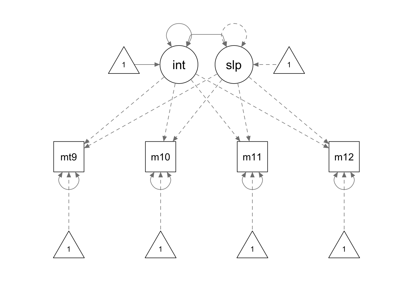
ms.model <- '

interc =~ 1*mathsc9 + 1*mathsc10 + 1*mathsc11 + 1*mathsc12
slope =~ 0*mathsc9 + 1*mathsc10 + 2*mathsc11 + 3*mathsc12

# constrain the intercept variance

interc ~~ 0*interc

'

ms.fit <- growth(ms.model, sample.cov = covmat, sample.mean = smeans, sample.nobs = 1000)

summary(ms.fit, fit.measures = T, standardized = F)
## lavaan 0.6.15 ended normally after 28 iterations
##
## Estimator ML
## Optimization method NLMINB
## Number of model parameters 8
##
## Number of observations 1000
##
## Model Test User Model:
##
## Test statistic 702.147
## Degrees of freedom 6
## P-value (Chi-square) 0.000
##
## Model Test Baseline Model:
##
## Test statistic 3045.699
## Degrees of freedom 6
## P-value 0.000
##
## User Model versus Baseline Model:
##
## Comparative Fit Index (CFI) 0.771
## Tucker-Lewis Index (TLI) 0.771
##
## Loglikelihood and Information Criteria:
##
## Loglikelihood user model (H0) -5669.489
## Loglikelihood unrestricted model (H1) -5318.415
##
## Akaike (AIC) 11354.978
## Bayesian (BIC) 11394.240
## Sample-size adjusted Bayesian (SABIC) 11368.831
##
## Root Mean Square Error of Approximation:
##
## RMSEA 0.341
## 90 Percent confidence interval - lower 0.320
## 90 Percent confidence interval - upper 0.362
## P-value H_0: RMSEA <= 0.050 0.000
## P-value H_0: RMSEA >= 0.080 1.000
##
## Standardized Root Mean Square Residual:
##
## SRMR 0.250
##
## Parameter Estimates:
##
## Standard errors Standard
## Information Expected
## Information saturated (h1) model Structured
##
## Latent Variables:
## Estimate Std.Err z-value P(>|z|)
## interc =~
## mathsc9 1.000
## mathsc10 1.000
## mathsc11 1.000
## mathsc12 1.000
## slope =~
## mathsc9 0.000
## mathsc10 1.000
## mathsc11 2.000
## mathsc12 3.000
##
## Covariances:
## Estimate Std.Err z-value P(>|z|)
## interc ~~
## slope 0.326 0.015 22.081 0.000
##
## Intercepts:
## Estimate Std.Err z-value P(>|z|)
## .mathsc9 0.000
## .mathsc10 0.000
## .mathsc11 0.000
## .mathsc12 0.000
## interc 3.288 0.032 103.873 0.000
## slope 0.369 0.010 36.510 0.000
##
## Variances:
## Estimate Std.Err z-value P(>|z|)
## interc 0.000
## .mathsc9 1.983 0.077 25.651 0.000
## .mathsc10 1.108 0.046 23.986 0.000
## .mathsc11 0.248 0.024 10.533 0.000
## .mathsc12 0.671 0.036 18.834 0.000
## slope -0.126 0.009 -14.695 0.000Example: LGM with Parallel Stability
ps.model <- '

interc =~ 1*mathsc9 + 1*mathsc10 + 1*mathsc11 + 1*mathsc12
slope =~ 0*mathsc9 + 1*mathsc10 + 2*mathsc11 + 3*mathsc12

# constrain the slope variance

slope ~~ 0*slope

'

ps.fit <- growth(ps.model, sample.cov = covmat, sample.mean = smeans, sample.nobs = 1000)

summary(ps.fit, fit.measures = T, standardized = F)
## lavaan 0.6.15 ended normally after 31 iterations
##
## Estimator ML
## Optimization method NLMINB
## Number of model parameters 8
##
## Number of observations 1000
##
## Model Test User Model:
##
## Test statistic 33.540
## Degrees of freedom 6
## P-value (Chi-square) 0.000
##
## Model Test Baseline Model:
##
## Test statistic 3045.699
## Degrees of freedom 6
## P-value 0.000
##
## User Model versus Baseline Model:
##
## Comparative Fit Index (CFI) 0.991
## Tucker-Lewis Index (TLI) 0.991
##
## Loglikelihood and Information Criteria:
##
## Loglikelihood user model (H0) -5335.185
## Loglikelihood unrestricted model (H1) -5318.415
##
## Akaike (AIC) 10686.370
## Bayesian (BIC) 10725.632
## Sample-size adjusted Bayesian (SABIC) 10700.224
##
## Root Mean Square Error of Approximation:
##
## RMSEA 0.068
## 90 Percent confidence interval - lower 0.046
## 90 Percent confidence interval - upper 0.091
## P-value H_0: RMSEA <= 0.050 0.082
## P-value H_0: RMSEA >= 0.080 0.205
##
## Standardized Root Mean Square Residual:
##
## SRMR 0.023
##
## Parameter Estimates:
##
## Standard errors Standard
## Information Expected
## Information saturated (h1) model Structured
##
## Latent Variables:
## Estimate Std.Err z-value P(>|z|)
## interc =~
## mathsc9 1.000
## mathsc10 1.000
## mathsc11 1.000
## mathsc12 1.000
## slope =~
## mathsc9 0.000
## mathsc10 1.000
## mathsc11 2.000
## mathsc12 3.000
##
## Covariances:
## Estimate Std.Err z-value P(>|z|)
## interc ~~
## slope -0.008 0.012 -0.628 0.530
##
## Intercepts:
## Estimate Std.Err z-value P(>|z|)
## .mathsc9 0.000
## .mathsc10 0.000
## .mathsc11 0.000
## .mathsc12 0.000
## interc 3.285 0.042 77.429 0.000
## slope 0.367 0.010 37.045 0.000
##
## Variances:
## Estimate Std.Err z-value P(>|z|)
## slope 0.000
## .mathsc9 0.718 0.037 19.186 0.000
## .mathsc10 0.557 0.030 18.362 0.000
## .mathsc11 0.271 0.019 14.221 0.000
## .mathsc12 0.328 0.021 15.335 0.000
## interc 1.365 0.079 17.172 0.000Example: LGM with Strict Stability
ss.model <- '

interc =~ 1*mathsc9 + 1*mathsc10 + 1*mathsc11 + 1*mathsc12
slope =~ 0*mathsc9 + 1*mathsc10 + 2*mathsc11 + 3*mathsc12

# constrain the slope variance
slope ~~ 0*slope

# constrain the slope mean
slope ~ 0*1

'

ss.fit <- growth(ss.model, sample.cov = covmat, sample.mean = smeans, sample.nobs = 1000)

summary(ss.fit, fit.measures = T, standardized = F)
## lavaan 0.6.15 ended normally after 29 iterations
##
## Estimator ML
## Optimization method NLMINB
## Number of model parameters 7
##
## Number of observations 1000
##
## Model Test User Model:
##
## Test statistic 1090.050
## Degrees of freedom 7
## P-value (Chi-square) 0.000
##
## Model Test Baseline Model:
##
## Test statistic 3045.699
## Degrees of freedom 6
## P-value 0.000
##
## User Model versus Baseline Model:
##
## Comparative Fit Index (CFI) 0.644
## Tucker-Lewis Index (TLI) 0.695
##
## Loglikelihood and Information Criteria:
##
## Loglikelihood user model (H0) -5863.440
## Loglikelihood unrestricted model (H1) -5318.415
##
## Akaike (AIC) 11740.880
## Bayesian (BIC) 11775.235
## Sample-size adjusted Bayesian (SABIC) 11753.002
##
## Root Mean Square Error of Approximation:
##
## RMSEA 0.393
## 90 Percent confidence interval - lower 0.374
## 90 Percent confidence interval - upper 0.413
## P-value H_0: RMSEA <= 0.050 0.000
## P-value H_0: RMSEA >= 0.080 1.000
##
## Standardized Root Mean Square Residual:
##
## SRMR 0.194
##
## Parameter Estimates:
##
## Standard errors Standard
## Information Expected
## Information saturated (h1) model Structured
##
## Latent Variables:
## Estimate Std.Err z-value P(>|z|)
## interc =~
## mathsc9 1.000
## mathsc10 1.000
## mathsc11 1.000
## mathsc12 1.000
## slope =~
## mathsc9 0.000
## mathsc10 1.000
## mathsc11 2.000
## mathsc12 3.000
##
## Covariances:
## Estimate Std.Err z-value P(>|z|)
## interc ~~
## slope -0.004 0.016 -0.235 0.814
##
## Intercepts:
## Estimate Std.Err z-value P(>|z|)
## slope 0.000
## .mathsc9 0.000
## .mathsc10 0.000
## .mathsc11 0.000
## .mathsc12 0.000
## interc 3.979 0.038 104.030 0.000
##
## Variances:
## Estimate Std.Err z-value P(>|z|)
## slope 0.000
## .mathsc9 1.249 0.062 20.167 0.000
## .mathsc10 0.737 0.040 18.626 0.000
## .mathsc11 0.232 0.021 11.112 0.000
## .mathsc12 0.565 0.033 17.352 0.000
## interc 1.355 0.088 15.388 0.000Example: Multi-group LGM
Read the data
setwd(mypath)  # change it to the path of your own data folder

dat <- read.table("multisample_data.csv", sep = ",", header = F)
colnames(dat) <-c('read1', 'read2', 'read3', 'country')

dat$country <- as.factor(dat$country)
levels(dat$country) <- c("korean", "china")

# check the data
str(dat)
## 'data.frame': 182 obs. of 4 variables:
## $ read1 : int 25 23 27 25 23 12 15 26 22 27 ...
## $ read2 : int 26 28 27 25 26 10 13 24 26 27 ...
## $ read3 : int 26 24 30 26 21 17 19 21 26 29 ...
## $ country: Factor w/ 2 levels "korean","china": 1 1 1 1 1 1 1 1 1 1 ...summary(dat)## read1 read2 read3 country
## Min. : 3.00 Min. : 2.00 Min. : 1.00 korean:96
## 1st Qu.:12.00 1st Qu.:14.00 1st Qu.:16.00 china :86
## Median :18.00 Median :19.00 Median :20.00
## Mean :17.76 Mean :18.83 Mean :19.76
## 3rd Qu.:23.00 3rd Qu.:24.00 3rd Qu.:25.00
## Max. :30.00 Max. :30.00 Max. :30.00Fit the model to the data
##      [,1] [,2] [,3]
## [1,] 0.25 0.15 0.05
## [2,] 0.15 0.10 0.05
## [3,] 0.05 0.05 0.05
##      [,1] [,2] [,3]
## [1,] 0.25 0.15 0.05
## [2,] 0.15 0.10 0.05
## [3,] 0.05 0.05 0.05
##      [,1] [,2] [,3]
## [1,] 0.25 0.15 0.05
## [2,] 0.15 0.10 0.05
## [3,] 0.05 0.05 0.05
##      [,1] [,2] [,3]
## [1,] 0.25 0.15 0.05
## [2,] 0.15 0.10 0.05
## [3,] 0.05 0.05 0.05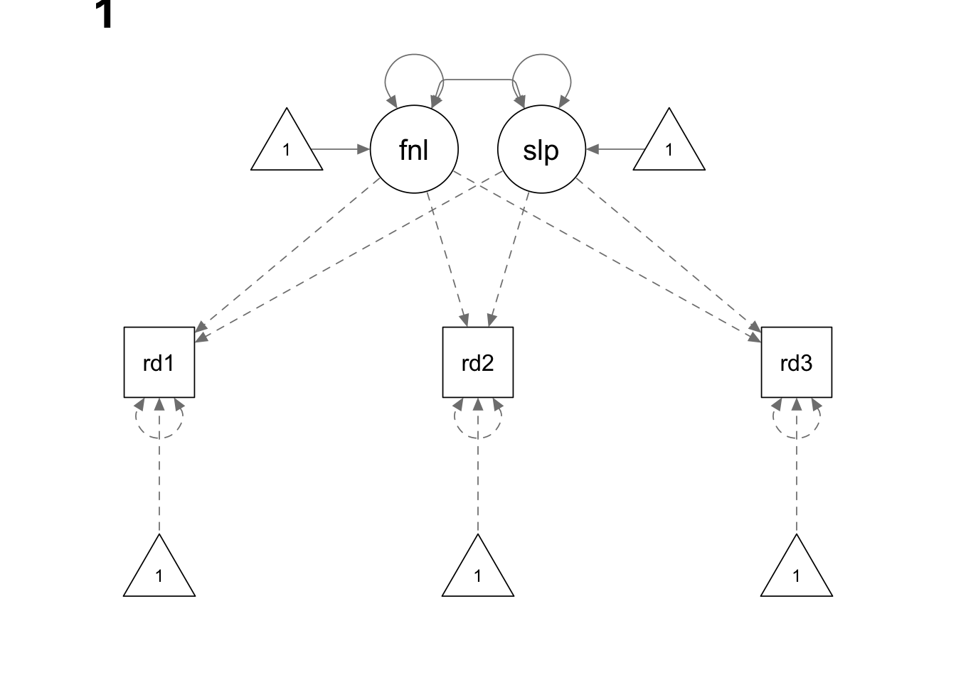
We use the sem() function here because we do not have
mean structure in this example. sem() function is thus more
flexible than the special function growth().
multigroup.model <- '

final =~ 1*read1 + 1*read2 + 1*read3
slope =~ -2*read1 + -1*read2 + 0*read3

final ~ c(ak, ac)*1
slope ~ c(bk, bc)*1

read1 ~ 0*1
read2 ~ 0*1
read3 ~ 0*1

final ~~ c(ck, cc)*final + slope
slope ~~ c(dk, dc)*slope

# test equality

adiff := ak - ac
bdiff := bk - bc
cdiff := ck - cc
ddiff := dk - dc

'

multigroup.fit <- sem(multigroup.model, data = dat, group = "country", group.equal = c("loadings"))
summary(multigroup.fit, fit.measures = T)
## lavaan 0.6.15 ended normally after 134 iterations
##
## Estimator ML
## Optimization method NLMINB
## Number of model parameters 16
##
## Number of observations per group:
## korean 96
## china 86
##
## Model Test User Model:
##
## Test statistic 2.375
## Degrees of freedom 2
## P-value (Chi-square) 0.305
## Test statistic for each group:
## korean 1.918
## china 0.456
##
## Model Test Baseline Model:
##
## Test statistic 370.321
## Degrees of freedom 6
## P-value 0.000
##
## User Model versus Baseline Model:
##
## Comparative Fit Index (CFI) 0.999
## Tucker-Lewis Index (TLI) 0.997
##
## Loglikelihood and Information Criteria:
##
## Loglikelihood user model (H0) -1614.597
## Loglikelihood unrestricted model (H1) -1613.410
##
## Akaike (AIC) 3261.194
## Bayesian (BIC) 3312.458
## Sample-size adjusted Bayesian (SABIC) 3261.784
##
## Root Mean Square Error of Approximation:
##
## RMSEA 0.045
## 90 Percent confidence interval - lower 0.000
## 90 Percent confidence interval - upper 0.218
## P-value H_0: RMSEA <= 0.050 0.384
## P-value H_0: RMSEA >= 0.080 0.508
##
## Standardized Root Mean Square Residual:
##
## SRMR 0.016
##
## Parameter Estimates:
##
## Standard errors Standard
## Information Expected
## Information saturated (h1) model Structured
##
##
## Group 1 [korean]:
##
## Latent Variables:
## Estimate Std.Err z-value P(>|z|)
## final =~
## read1 1.000
## read2 1.000
## read3 1.000
## slope =~
## read1 -2.000
## read2 -1.000
## read3 0.000
##
## Covariances:
## Estimate Std.Err z-value P(>|z|)
## final ~~
## slope -0.901 2.228 -0.404 0.686
##
## Intercepts:
## Estimate Std.Err z-value P(>|z|)
## final (ak) 20.809 0.585 35.600 0.000
## slope (bk) 0.716 0.200 3.573 0.000
## .read1 0.000
## .read2 0.000
## .read3 0.000
##
## Variances:
## Estimate Std.Err z-value P(>|z|)
## final (ck) 27.993 5.378 5.205 0.000
## slope (dk) 0.523 1.903 0.275 0.783
## .read1 7.749 4.067 1.905 0.057
## .read2 5.861 1.958 2.994 0.003
## .read3 5.680 3.643 1.559 0.119
##
##
## Group 2 [china]:
##
## Latent Variables:
## Estimate Std.Err z-value P(>|z|)
## final =~
## read1 1.000
## read2 1.000
## read3 1.000
## slope =~
## read1 -2.000
## read2 -1.000
## read3 0.000
##
## Covariances:
## Estimate Std.Err z-value P(>|z|)
## final ~~
## slope 1.945 3.737 0.520 0.603
##
## Intercepts:
## Estimate Std.Err z-value P(>|z|)
## final (ac) 18.611 0.752 24.740 0.000
## slope (bc) 1.250 0.305 4.102 0.000
## .read1 0.000
## .read2 0.000
## .read3 0.000
##
## Variances:
## Estimate Std.Err z-value P(>|z|)
## final (cc) 36.539 8.741 4.180 0.000
## slope (dc) 3.378 3.361 1.005 0.315
## .read1 4.787 6.642 0.721 0.471
## .read2 15.112 3.817 3.959 0.000
## .read3 14.904 7.108 2.097 0.036
##
## Defined Parameters:
## Estimate Std.Err z-value P(>|z|)
## adiff 2.197 0.953 2.306 0.021
## bdiff -0.534 0.365 -1.465 0.143
## cdiff -8.546 10.263 -0.833 0.405
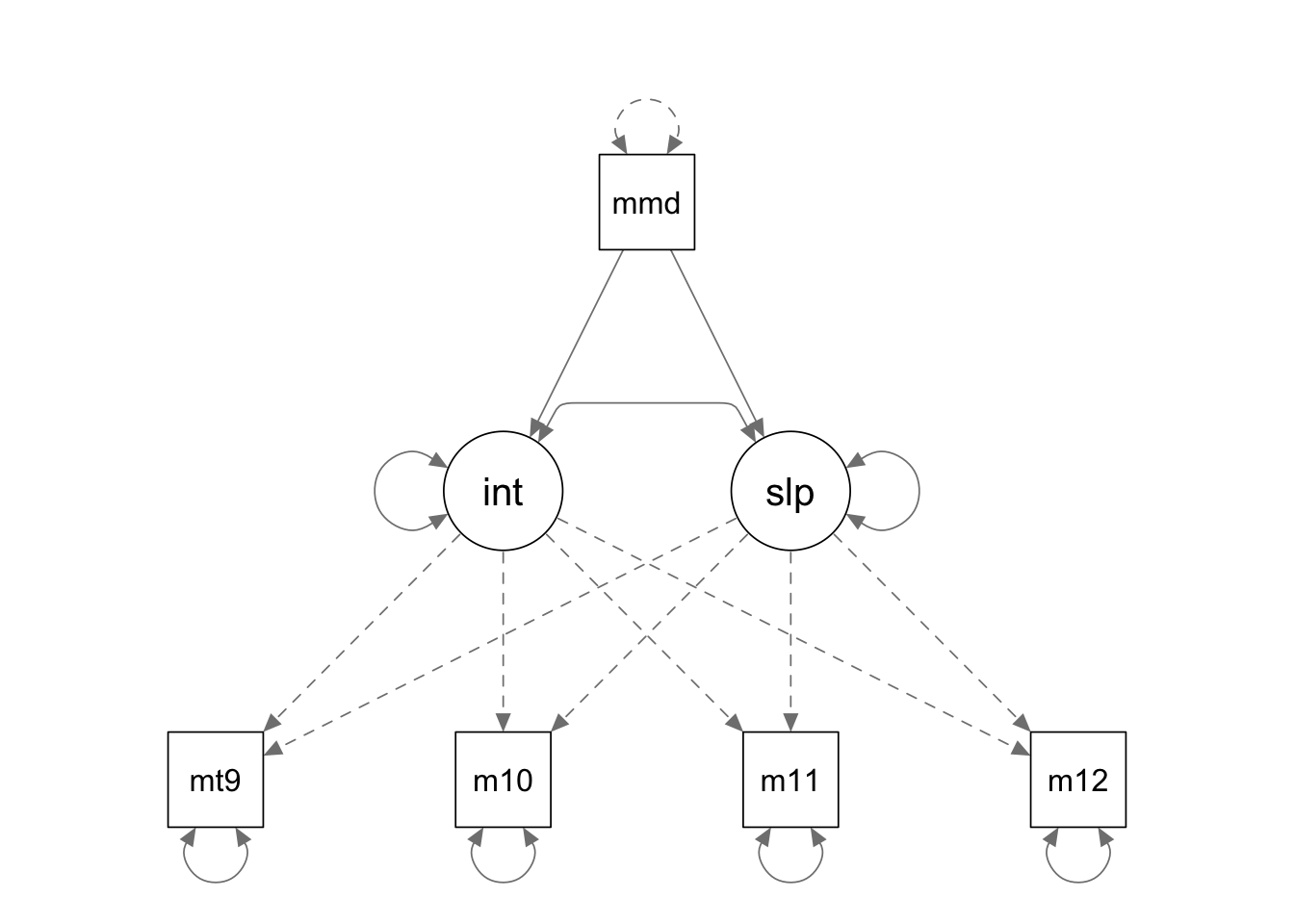
## ddiff -2.855 3.862 -0.739 0.460Example: Conditional LGM
In this example we will fit a linear LGM with a predictor variable. You may have noticed that we do not have sample means in this example. It is fine because what is of focal interest here is the path coefficients from the predictor variable to the latent variables.
Read the data
lower <- '
2.041
1.392  1.901
1.366  1.352  1.665
1.249  1.303  1.348  1.599
1.212  1.923  2.233  2.943  7.290
'

covmat <- getCov(lower)
colnames(covmat) <- c(paste0('mathsc', 9:12), "momed")
rownames(covmat) <- colnames(covmat)
Fit the model to the data
We use the sem() function here because we do not have
mean structure in this example. sem() function is thus more
flexible than the special function growth().
conditional.model <- '
interc =~ 1*mathsc9 + 1*mathsc10 + 1*mathsc11 + 1*mathsc12
slope =~ 0*mathsc9 + 1*mathsc10 + 2*mathsc11 + 3*mathsc12

interc ~ momed
slope ~ momed
'

conditional.fit <- sem(conditional.model, sample.cov = covmat, sample.nobs = 1000)
summary(conditional.fit, fit.measures = T, standardized = T)
## lavaan 0.6.15 ended normally after 58 iterations
##
## Estimator ML
## Optimization method NLMINB
## Number of model parameters 9
##
## Number of observations 1000
##
## Model Test User Model:
##
## Test statistic 31.482
## Degrees of freedom 5
## P-value (Chi-square) 0.000
##
## Model Test Baseline Model:
##
## Test statistic 5343.753
## Degrees of freedom 10
## P-value 0.000
##
## User Model versus Baseline Model:
##
## Comparative Fit Index (CFI) 0.995
## Tucker-Lewis Index (TLI) 0.990
##
## Loglikelihood and Information Criteria:
##
## Loglikelihood user model (H0) -4185.129
## Loglikelihood unrestricted model (H1) -4169.388
##
## Akaike (AIC) 8388.259
## Bayesian (BIC) 8432.428
## Sample-size adjusted Bayesian (SABIC) 8403.844
##
## Root Mean Square Error of Approximation:
##
## RMSEA 0.073
## 90 Percent confidence interval - lower 0.050
## 90 Percent confidence interval - upper 0.098
## P-value H_0: RMSEA <= 0.050 0.052
## P-value H_0: RMSEA >= 0.080 0.344
##
## Standardized Root Mean Square Residual:
##
## SRMR 0.022
##
## Parameter Estimates:
##
## Standard errors Standard
## Information Expected
## Information saturated (h1) model Structured
##
## Latent Variables:
## Estimate Std.Err z-value P(>|z|) Std.lv Std.all
## interc =~
## mathsc9 1.000 1.245 0.884
## mathsc10 1.000 1.245 0.884
## mathsc11 1.000 1.245 0.955
## mathsc12 1.000 1.245 0.990
## slope =~
## mathsc9 0.000 0.000 0.000
## mathsc10 1.000 0.240 0.170
## mathsc11 2.000 0.480 0.368
## mathsc12 3.000 0.720 0.573
##
## Regressions:
## Estimate Std.Err z-value P(>|z|) Std.lv Std.all
## interc ~
## momed 0.168 0.015 11.171 0.000 0.135 0.364
## slope ~
## momed 0.077 0.003 24.985 0.000 0.323 0.871
##
## Covariances:
## Estimate Std.Err z-value P(>|z|) Std.lv Std.all
## .interc ~~
## .slope -0.200 0.016 -12.412 0.000 -1.463 -1.463
##
## Variances:
## Estimate Std.Err z-value P(>|z|) Std.lv Std.all
## .mathsc9 0.433 0.031 13.863 0.000 0.433 0.219
## .mathsc10 0.586 0.030 19.537 0.000 0.586 0.296
## .mathsc11 0.338 0.018 18.503 0.000 0.338 0.199
## .mathsc12 0.144 0.012 12.423 0.000 0.144 0.091
## .interc 1.343 0.076 17.765 0.000 0.867 0.867
## .slope 0.014 0.005 3.009 0.003 0.242 0.242Example: Conditional Multigroup LGM
Read the data
setwd(mypath)  # change it to the path of your own data folder

dat <- read.table("predictor2_data.csv", sep = ",", header = F)
colnames(dat) <-c(paste0('math', 7:10), 'sex', 'quant')

dat$sex <- as.factor(dat$sex)
levels(dat$sex) <- c("female", "male")

# check the data
str(dat)
## 'data.frame': 1994 obs. of 6 variables:
## $ math7 : num 62 61.2 59.4 54.6 62 ...
## $ math8 : num 62.3 60.3 54.8 51.2 61 ...
## $ math9 : num 69 64.4 59.4 64.1 62.4 ...
## $ math10: num 68.4 65.3 63 62.3 61.5 ...
## $ sex : Factor w/ 2 levels "female","male": 2 1 2 2 1 1 1 2 2 2 ...
## $ quant : num 40.9 49.6 47.2 46.4 31.4 ...summary(dat)## math7 math8 math9 math10
## Min. :28.19 Min. :23.85 Min. :28.61 Min. :28.16
## 1st Qu.:45.49 1st Qu.:48.42 1st Qu.:51.08 1st Qu.:53.29
## Median :53.15 Median :55.75 Median :59.31 Median :62.88
## Mean :52.20 Mean :54.80 Mean :58.60 Mean :61.42
## 3rd Qu.:59.62 3rd Qu.:61.79 3rd Qu.:66.77 3rd Qu.:69.95
## Max. :83.97 Max. :84.17 Max. :88.88 Max. :93.96
## sex quant
## female:1006 Min. :19.37
## male : 988 1st Qu.:43.36
## Median :50.39
## Mean :50.32
## 3rd Qu.:56.83
## Max. :82.28Fit the model to the data

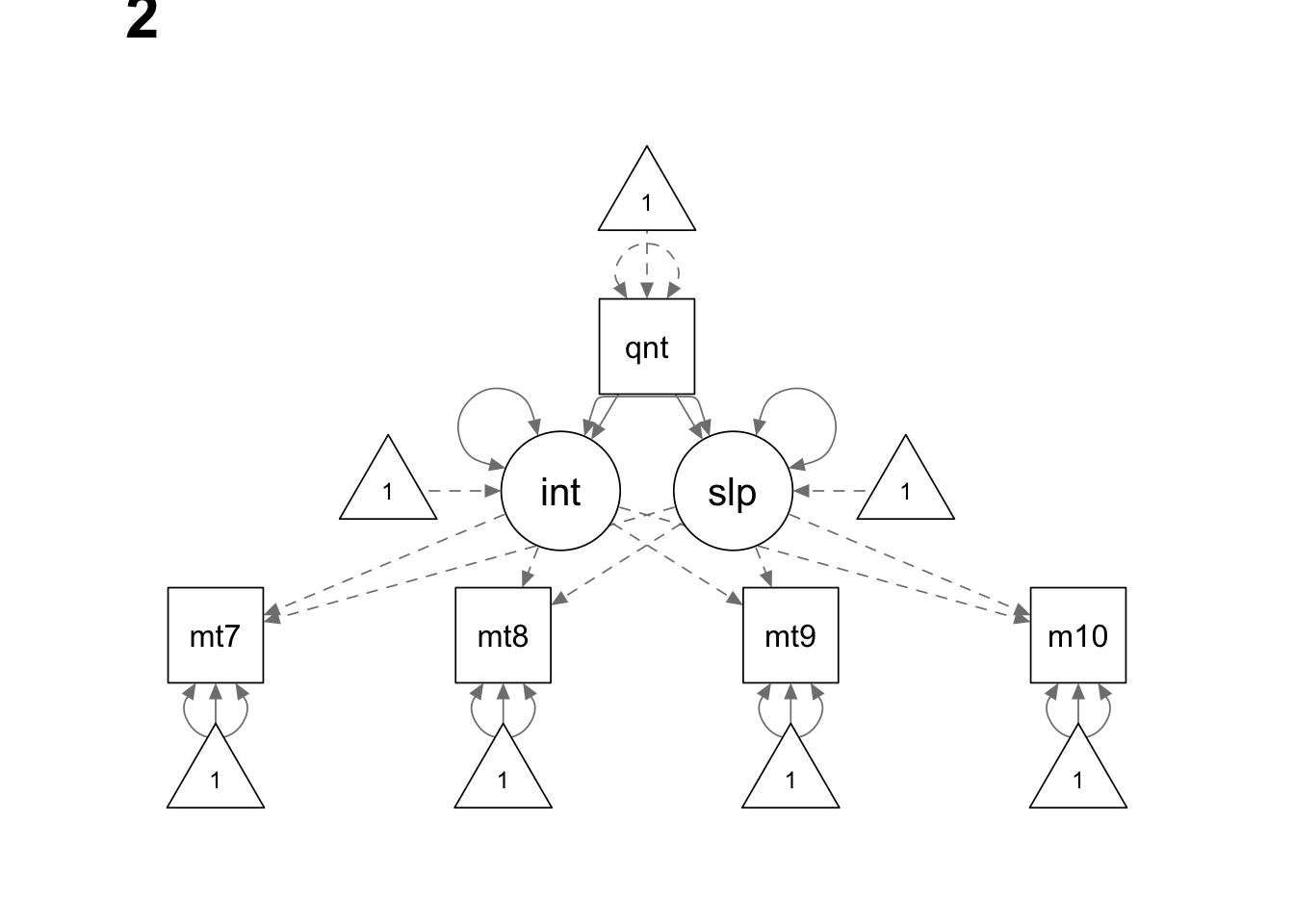
We use the sem() function here because we do not have
mean structure in this example. sem() function is thus more
flexible than the special function growth().
model <- '

interc =~ 1*math7 + 1*math8 + 1*math9 + 1*math10
slope =~ 0*math7 + 1*math8 + 2*math9 + 3*math10

math7 ~ c(a, a)*1
math8 ~ c(b, b)*1
math9 ~ c(c, c)*1
math10 ~ c(d, d)*1

interc ~ c(NA, 0)*1
slope ~ c(NA, 0)*1

interc ~ c(am, af)*quant
slope ~ c(bm, bf)*quant

interc ~~ slope

# test the equality constraints

adiff := af - am
bdiff := bf - bm

'

fit <- sem(model, dat, group = "sex", group.equal = c("loadings"))
summary(fit, fit.measures = T)
## lavaan 0.6.15 ended normally after 163 iterations
##
## Estimator ML
## Optimization method NLMINB
## Number of model parameters 28
## Number of equality constraints 4
##
## Number of observations per group:
## male 988
## female 1006
##
## Model Test User Model:
##
## Test statistic 25.963
## Degrees of freedom 12
## P-value (Chi-square) 0.011
## Test statistic for each group:
## male 8.137
## female 17.826
##
## Model Test Baseline Model:
##
## Test statistic 7556.622
## Degrees of freedom 20
## P-value 0.000
##
## User Model versus Baseline Model:
##
## Comparative Fit Index (CFI) 0.998
## Tucker-Lewis Index (TLI) 0.997
##
## Loglikelihood and Information Criteria:
##
## Loglikelihood user model (H0) -26549.655
## Loglikelihood unrestricted model (H1) -26536.674
##
## Akaike (AIC) 53147.311
## Bayesian (BIC) 53281.660
## Sample-size adjusted Bayesian (SABIC) 53205.411
##
## Root Mean Square Error of Approximation:
##
## RMSEA 0.034
## 90 Percent confidence interval - lower 0.016
## 90 Percent confidence interval - upper 0.052
## P-value H_0: RMSEA <= 0.050 0.922
## P-value H_0: RMSEA >= 0.080 0.000
##
## Standardized Root Mean Square Residual:
##
## SRMR 0.012
##
## Parameter Estimates:
##
## Standard errors Standard
## Information Expected
## Information saturated (h1) model Structured
##
##
## Group 1 [male]:
##
## Latent Variables:
## Estimate Std.Err z-value P(>|z|)
## interc =~
## math7 1.000
## math8 1.000
## math9 1.000
## math10 1.000
## slope =~
## math7 0.000
## math8 1.000
## math9 2.000
## math10 3.000
##
## Regressions:
## Estimate Std.Err z-value P(>|z|)
## interc ~
## quant (am) 0.008 0.030 0.252 0.801
## slope ~
## quant (bm) 0.006 0.009 0.744 0.457
##
## Covariances:
## Estimate Std.Err z-value P(>|z|)
## .interc ~~
## .slope 4.599 0.880 5.226 0.000
##
## Intercepts:
## Estimate Std.Err z-value P(>|z|)
## .math7 (a) 51.665 1.549 33.364 0.000
## .math8 (b) 54.763 1.575 34.767 0.000
## .math9 (c) 59.053 1.711 34.519 0.000
## .math10 (d) 62.368 1.933 32.261 0.000
## .interc 0.126 2.196 0.057 0.954
## .slope -0.903 0.620 -1.457 0.145
##
## Variances:
## Estimate Std.Err z-value P(>|z|)
## .math7 13.213 1.378 9.588 0.000
## .math8 15.973 1.015 15.732 0.000
## .math9 18.370 1.223 15.020 0.000
## .math10 32.554 2.364 13.770 0.000
## .interc 74.843 3.907 19.158 0.000
## .slope 3.035 0.401 7.571 0.000
##
##
## Group 2 [female]:
##
## Latent Variables:
## Estimate Std.Err z-value P(>|z|)
## interc =~
## math7 1.000
## math8 1.000
## math9 1.000
## math10 1.000
## slope =~
## math7 0.000
## math8 1.000
## math9 2.000
## math10 3.000
##
## Regressions:
## Estimate Std.Err z-value P(>|z|)
## interc ~
## quant (af) 0.011 0.030 0.375 0.708
## slope ~
## quant (bf) -0.008 0.008 -1.013 0.311
##
## Covariances:
## Estimate Std.Err z-value P(>|z|)
## .interc ~~
## .slope 3.975 0.878 4.526 0.000
##
## Intercepts:
## Estimate Std.Err z-value P(>|z|)
## .math7 (a) 51.665 1.549 33.364 0.000
## .math8 (b) 54.763 1.575 34.767 0.000
## .math9 (c) 59.053 1.711 34.519 0.000
## .math10 (d) 62.368 1.933 32.261 0.000
## .interc 0.000
## .slope 0.000
##
## Variances:
## Estimate Std.Err z-value P(>|z|)
## .math7 17.135 1.447 11.843 0.000
## .math8 13.632 0.935 14.574 0.000
## .math9 18.528 1.210 15.306 0.000
## .math10 36.548 2.434 15.018 0.000
## .interc 79.388 4.134 19.202 0.000
## .slope 2.165 0.391 5.543 0.000
##
## Defined Parameters:
## Estimate Std.Err z-value P(>|z|)
## adiff 0.004 0.043 0.088 0.930
## bdiff -0.015 0.012 -1.238 0.216© Copyright 2024 @Yi Feng and @Gregory R. Hancock.