Latent Growth Models Extensions
In this tutorial, we are going to use the R package
lavaan for advanced latent growth models and package
OpenMx for mixture growth models.
Load the pacakges
library(lavaan)
library(semPlot)
library(OpenMx)
library(readr)
Example: LGM with time dependent covariates
The data for this example are from 324 non-native English speakers, whose reading ability and writing ability have been measured at three equally spaced time points (1 month apart).
Read the data
lower <- '
42.916
32.060  39.350
29.666  28.796  37.428
18.070  17.553  16.614  20.924
17.863  17.192  16.142  14.665  17.987
17.294  17.261  17.032  14.893  13.786  18.103
'

covmat <- getCov(lower)
smeans <- c(17.080, 18.404, 19.228, 18.590, 19.352, 20.265)

rownames(covmat) <- colnames(covmat) <- c(paste0("read", 1:3), paste0("write", 1:3))
Fit the model
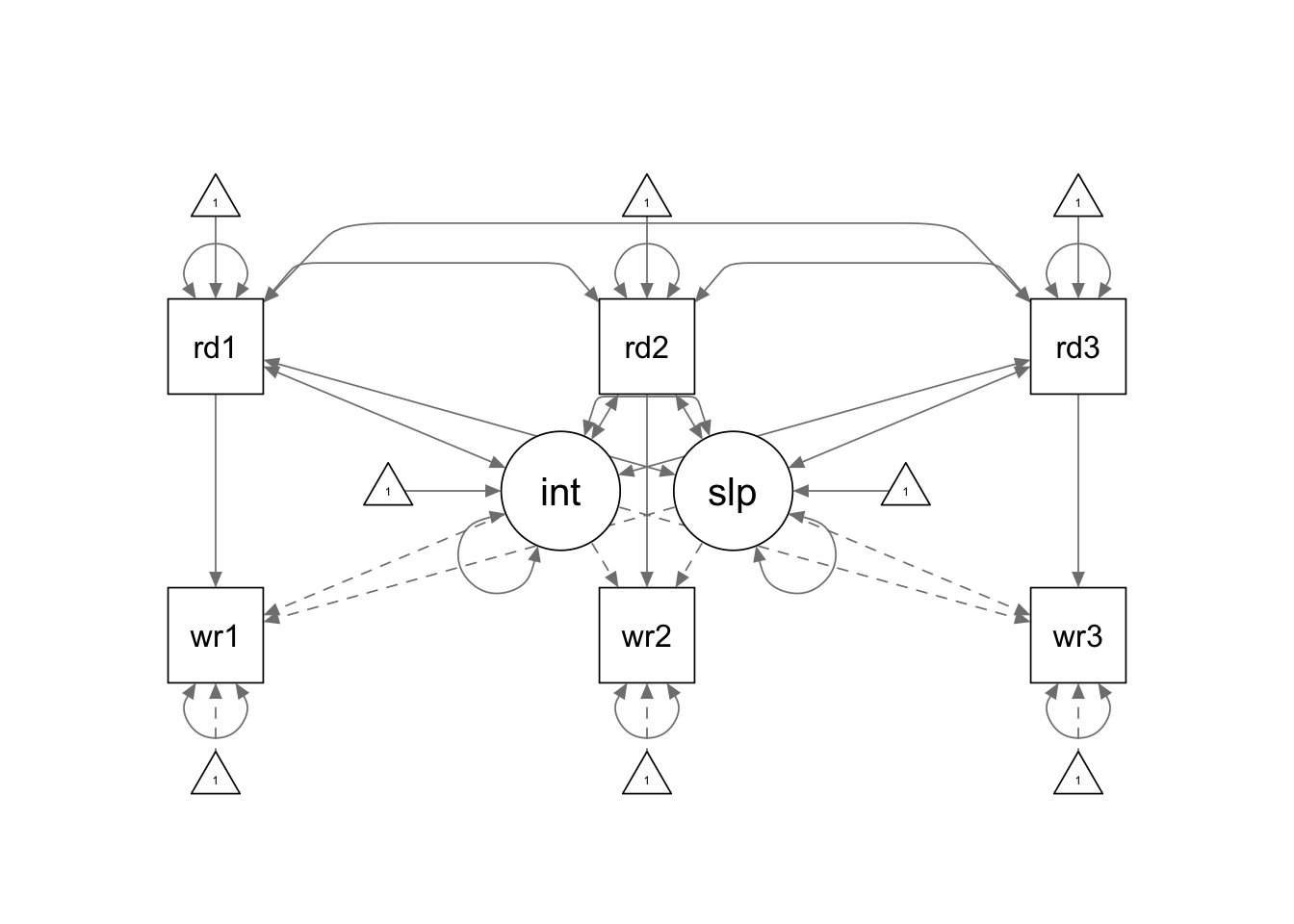
No special syntax is required for you to fit a LGM with time
dependent covariates. You only need to correctly specify the covariance
structure and mean structure for your model using the regular
lavaan model syntax. This is another example showing you
that it is more important to have a good understanding of the models
before you translate it into programming language. :)
tdc.model <- '

# latent intercept and slope

interc =~ 1*write1 + 1*write2 + 1*write3
slope =~ 0*write1 + 1*write2 + 2*write3

# path coefficients

write1 ~ read1
write2 ~ read2
write3 ~ read3

# covariances

read1 ~~ interc + slope + read2 + read3
read2 ~~ interc + slope + read3
read3 ~~ interc + slope

# means

read1 ~ 1
read2 ~ 1
read3 ~ 1

'

tdc.fit <- growth(tdc.model, sample.cov = covmat, sample.mean = smeans, sample.nobs = 324)
summary(tdc.fit, fit.measures = T, standardized = T)
## lavaan 0.6.15 ended normally after 165 iterations
##
## Estimator ML
## Optimization method NLMINB
## Number of model parameters 26
##
## Number of observations 324
##
## Model Test User Model:
##
## Test statistic 0.189
## Degrees of freedom 1
## P-value (Chi-square) 0.664
##
## Model Test Baseline Model:
##
## Test statistic 1522.714
## Degrees of freedom 15
## P-value 0.000
##
## User Model versus Baseline Model:
##
## Comparative Fit Index (CFI) 1.000
## Tucker-Lewis Index (TLI) 1.008
##
## Loglikelihood and Information Criteria:
##
## Loglikelihood user model (H0) -5214.836
## Loglikelihood unrestricted model (H1) -5214.742
##
## Akaike (AIC) 10481.672
## Bayesian (BIC) 10579.972
## Sample-size adjusted Bayesian (SABIC) 10497.502
##
## Root Mean Square Error of Approximation:
##
## RMSEA 0.000
## 90 Percent confidence interval - lower 0.000
## 90 Percent confidence interval - upper 0.112
## P-value H_0: RMSEA <= 0.050 0.770
## P-value H_0: RMSEA >= 0.080 0.127
##
## Standardized Root Mean Square Residual:
##
## SRMR 0.005
##
## Parameter Estimates:
##
## Standard errors Standard
## Information Expected
## Information saturated (h1) model Structured
##
## Latent Variables:
## Estimate Std.Err z-value P(>|z|) Std.lv Std.all
## interc =~
## write1 1.000 4.180 0.919
## write2 1.000 4.180 0.982
## write3 1.000 4.180 0.987
## slope =~
## write1 0.000 NA NA
## write2 1.000 NA NA
## write3 2.000 NA NA
##
## Regressions:
## Estimate Std.Err z-value P(>|z|) Std.lv Std.all
## write1 ~
## read1 -0.077 0.076 -1.012 0.312 -0.077 -0.110
## write2 ~
## read2 0.001 0.039 0.032 0.975 0.001 0.002
## write3 ~
## read3 0.080 0.071 1.135 0.256 0.080 0.116
##
## Covariances:
## Estimate Std.Err z-value P(>|z|) Std.lv Std.all
## interc ~~
## read1 21.146 3.637 5.814 0.000 5.059 0.773
## slope ~~
## read1 -3.197 2.310 -1.384 0.166 -5.913 -0.904
## read1 ~~
## read2 31.961 2.887 11.072 0.000 31.961 0.780
## read3 29.574 2.762 10.709 0.000 29.574 0.740
## interc ~~
## read2 19.790 3.129 6.326 0.000 4.735 0.756
## slope ~~
## read2 -2.506 1.943 -1.289 0.197 -4.634 -0.740
## read2 ~~
## read3 28.707 2.657 10.803 0.000 28.707 0.750
## interc ~~
## read3 18.664 2.943 6.342 0.000 4.466 0.731
## slope ~~
## read3 -2.405 2.125 -1.132 0.258 -4.447 -0.728
## interc ~~
## slope -1.477 1.567 -0.942 0.346 -0.653 -0.653
##
## Intercepts:
## Estimate Std.Err z-value P(>|z|) Std.lv Std.all
## read1 17.080 0.363 47.003 0.000 17.080 2.611
## read2 18.404 0.348 52.891 0.000 18.404 2.938
## read3 19.228 0.339 56.660 0.000 19.228 3.148
## .write1 0.000 0.000 0.000
## .write2 0.000 0.000 0.000
## .write3 0.000 0.000 0.000
## interc 19.907 1.321 15.070 0.000 4.763 4.763
## slope -0.588 1.115 -0.528 0.598 NA NA
##
## Variances:
## Estimate Std.Err z-value P(>|z|) Std.lv Std.all
## .write1 6.218 1.046 5.945 0.000 6.218 0.300
## .write2 3.864 0.486 7.942 0.000 3.864 0.213
## .write3 5.061 0.913 5.541 0.000 5.061 0.282
## read1 42.784 3.361 12.728 0.000 42.784 1.000
## read2 39.229 3.082 12.728 0.000 39.229 1.000
## read3 37.312 2.932 12.728 0.000 37.312 1.000
## interc 17.469 3.596 4.858 0.000 1.000 1.000
## slope -0.292 0.591 -0.495 0.621 NA NAExample: Multiple Domain Models
Read the data
setwd(mypath)  # set working directory to where the data file is stored

dat <- read.delim("multiple_domain_data.txt", sep = '\t', header = F)
colnames(dat) <- c('read1', 'read2', 'read3', 'list1', 'list2', 'list3',
                        'speak1', 'speak2', 'speak3', 'write1', 'write2', 'write3')

str(dat)
## 'data.frame': 170 obs. of 12 variables:
## $ read1 : int 22 19 24 21 24 17 14 30 19 11 ...
## $ read2 : int 24 19 26 24 26 21 19 29 23 6 ...
## $ read3 : int 23 17 30 27 28 20 20 29 23 13 ...
## $ list1 : int 28 18 27 18 29 18 14 27 13 15 ...
## $ list2 : int 30 16 30 20 28 16 7 18 10 8 ...
## $ list3 : int 29 17 27 18 26 17 10 24 17 19 ...
## $ speak1: int 23 19 24 22 17 14 14 23 17 23 ...
## $ speak2: int 23 18 24 17 18 17 10 22 17 22 ...
## $ speak3: int 23 18 29 17 19 15 10 23 18 24 ...
## $ write1: int 25 17 21 18 20 21 14 22 17 17 ...
## $ write2: int 22 20 24 21 20 17 18 25 20 18 ...
## $ write3: int 21 25 27 22 22 21 18 22 17 18 ...summary(dat)## read1 read2 read3 list1
## Min. : 0.00 Min. : 3.00 Min. : 4.00 Min. : 1.00
## 1st Qu.:13.00 1st Qu.:14.00 1st Qu.:16.00 1st Qu.:13.00
## Median :17.00 Median :19.00 Median :20.00 Median :17.00
## Mean :17.38 Mean :18.55 Mean :19.55 Mean :16.56
## 3rd Qu.:22.00 3rd Qu.:23.00 3rd Qu.:23.00 3rd Qu.:21.00
## Max. :30.00 Max. :30.00 Max. :30.00 Max. :30.00
## list2 list3 speak1 speak2
## Min. : 1.00 Min. : 1.00 Min. : 0.00 Min. : 5.00
## 1st Qu.:14.00 1st Qu.:15.00 1st Qu.:15.00 1st Qu.:17.00
## Median :18.00 Median :19.00 Median :18.00 Median :18.00
## Mean :17.63 Mean :18.58 Mean :17.96 Mean :18.73
## 3rd Qu.:21.75 3rd Qu.:23.00 3rd Qu.:20.00 3rd Qu.:22.00
## Max. :30.00 Max. :30.00 Max. :28.00 Max. :27.00
## speak3 write1 write2 write3
## Min. :10.00 Min. : 7.00 Min. : 8.00 Min. : 7.00
## 1st Qu.:17.00 1st Qu.:15.00 1st Qu.:17.00 1st Qu.:18.00
## Median :19.00 Median :20.00 Median :20.00 Median :20.50
## Mean :19.24 Mean :18.59 Mean :19.58 Mean :20.11
## 3rd Qu.:22.00 3rd Qu.:21.00 3rd Qu.:22.00 3rd Qu.:22.00
## Max. :29.00 Max. :30.00 Max. :28.00 Max. :29.00Unstructured Growth
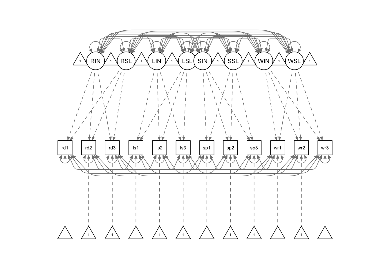
md.model <- '

RINT =~ 1*read1 + 1*read2 + 1*read3
RSLOPE =~ 0*read1 + 1*read2 + 2*read3

LINT =~ 1*list1 + 1*list2 + 1*list3
LSLOPE =~ 0*list1 + 1*list2 + 2*list3

SINT =~ 1*speak1 + 1*speak2 + 1*speak3
SSLOPE =~ 0*speak1 + 1*speak2 + 2*speak3

WINT =~ 1*write1 + 1*write2 + 1*write3
WSLOPE =~ 0*write1 + 1*write2 + 2*write3


RINT ~ 1
RSLOPE ~ 1
LINT ~ 1
LSLOPE ~ 1
SINT ~ 1
SSLOPE ~ 1
WINT ~ 1
WSLOPE ~ 1

read1 ~ 0*1
read2 ~ 0*1
read3 ~ 0*1

list1 ~ 0*1
list2 ~ 0*1
list3 ~ 0*1

speak1 ~ 0*1
speak2 ~ 0*1
speak3 ~ 0*1

write1 ~ 0*1
write2 ~ 0*1
write3 ~ 0*1


read1 ~~ list1 + speak1 + write1
read2 ~~ list2 + speak2 + write2
read3 ~~ list3 + speak3 + write3

list1 ~~ speak1 + write1
list2 ~~ speak2 + write2
list3 ~~ speak3 + write3

speak1 ~~ write1
speak2 ~~ write2
speak3 ~~ write3


'

md.fit <- sem(md.model, dat)
summary(md.fit, fit.measures = T)
## lavaan 0.6.15 ended normally after 394 iterations
##
## Estimator ML
## Optimization method NLMINB
## Number of model parameters 74
##
## Number of observations 170
##
## Model Test User Model:
##
## Test statistic 15.567
## Degrees of freedom 16
## P-value (Chi-square) 0.484
##
## Model Test Baseline Model:
##
## Test statistic 1711.627
## Degrees of freedom 66
## P-value 0.000
##
## User Model versus Baseline Model:
##
## Comparative Fit Index (CFI) 1.000
## Tucker-Lewis Index (TLI) 1.001
##
## Loglikelihood and Information Criteria:
##
## Loglikelihood user model (H0) -5306.076
## Loglikelihood unrestricted model (H1) -5298.293
##
## Akaike (AIC) 10760.153
## Bayesian (BIC) 10992.202
## Sample-size adjusted Bayesian (SABIC) 10757.891
##
## Root Mean Square Error of Approximation:
##
## RMSEA 0.000
## 90 Percent confidence interval - lower 0.000
## 90 Percent confidence interval - upper 0.069
## P-value H_0: RMSEA <= 0.050 0.827
## P-value H_0: RMSEA >= 0.080 0.019
##
## Standardized Root Mean Square Residual:
##
## SRMR 0.029
##
## Parameter Estimates:
##
## Standard errors Standard
## Information Expected
## Information saturated (h1) model Structured
##
## Latent Variables:
## Estimate Std.Err z-value P(>|z|)
## RINT =~
## read1 1.000
## read2 1.000
## read3 1.000
## RSLOPE =~
## read1 0.000
## read2 1.000
## read3 2.000
## LINT =~
## list1 1.000
## list2 1.000
## list3 1.000
## LSLOPE =~
## list1 0.000
## list2 1.000
## list3 2.000
## SINT =~
## speak1 1.000
## speak2 1.000
## speak3 1.000
## SSLOPE =~
## speak1 0.000
## speak2 1.000
## speak3 2.000
## WINT =~
## write1 1.000
## write2 1.000
## write3 1.000
## WSLOPE =~
## write1 0.000
## write2 1.000
## write3 2.000
##
## Covariances:
## Estimate Std.Err z-value P(>|z|)
## .read1 ~~
## .list1 2.930 2.375 1.234 0.217
## .speak1 0.123 1.424 0.087 0.931
## .write1 -1.807 1.644 -1.100 0.272
## .read2 ~~
## .list2 0.078 1.332 0.059 0.953
## .speak2 -0.147 0.686 -0.214 0.831
## .write2 0.653 0.833 0.784 0.433
## .read3 ~~
## .list3 0.539 2.210 0.244 0.807
## .speak3 0.687 1.228 0.559 0.576
## .write3 -0.698 1.438 -0.486 0.627
## .list1 ~~
## .speak1 0.186 1.443 0.129 0.898
## .write1 2.345 1.608 1.458 0.145
## .list2 ~~
## .speak2 0.432 0.796 0.543 0.587
## .write2 -0.534 0.895 -0.596 0.551
## .list3 ~~
## .speak3 -0.479 1.337 -0.358 0.720
## .write3 0.716 1.483 0.482 0.629
## .speak1 ~~
## .write1 2.183 1.020 2.141 0.032
## .speak2 ~~
## .write2 -0.291 0.484 -0.601 0.548
## .speak3 ~~
## .write3 0.244 0.894 0.273 0.785
## RINT ~~
## RSLOPE -2.156 1.846 -1.168 0.243
## LINT 17.235 3.569 4.829 0.000
## LSLOPE 1.510 1.540 0.980 0.327
## SINT 8.868 2.174 4.078 0.000
## SSLOPE -0.483 0.870 -0.555 0.579
## WINT 17.697 2.602 6.801 0.000
## WSLOPE -1.338 0.998 -1.341 0.180
## RSLOPE ~~
## LINT -0.583 1.458 -0.400 0.689
## LSLOPE 0.645 1.115 0.578 0.563
## SINT -0.609 0.908 -0.671 0.502
## SSLOPE -0.090 0.646 -0.139 0.889
## WINT -2.329 1.024 -2.275 0.023
## WSLOPE 0.940 0.749 1.255 0.209
## LINT ~~
## LSLOPE -1.869 1.808 -1.034 0.301
## SINT 13.981 2.243 6.232 0.000
## SSLOPE -0.407 0.851 -0.478 0.633
## WINT 14.656 2.489 5.888 0.000
## WSLOPE -0.555 0.960 -0.578 0.563
## LSLOPE ~~
## SINT -0.684 0.948 -0.722 0.471
## SSLOPE 0.396 0.677 0.584 0.559
## WINT -0.040 1.037 -0.039 0.969
## WSLOPE 0.087 0.748 0.117 0.907
## SINT ~~
## SSLOPE -0.492 0.649 -0.758 0.448
## WINT 9.779 1.615 6.055 0.000
## WSLOPE -0.228 0.613 -0.372 0.710
## SSLOPE ~~
## WINT -0.177 0.601 -0.295 0.768
## WSLOPE -0.101 0.465 -0.216 0.829
## WINT ~~
## WSLOPE -0.472 0.778 -0.607 0.544
##
## Intercepts:
## Estimate Std.Err z-value P(>|z|)
## RINT 17.383 0.480 36.192 0.000
## RSLOPE 1.091 0.171 6.377 0.000
## LINT 16.626 0.452 36.807 0.000
## LSLOPE 0.984 0.186 5.285 0.000
## SINT 18.058 0.302 59.726 0.000
## SSLOPE 0.611 0.104 5.859 0.000
## WINT 18.717 0.325 57.663 0.000
## WSLOPE 0.721 0.117 6.186 0.000
## .read1 0.000
## .read2 0.000
## .read3 0.000
## .list1 0.000
## .list2 0.000
## .list3 0.000
## .speak1 0.000
## .speak2 0.000
## .speak3 0.000
## .write1 0.000
## .write2 0.000
## .write3 0.000
##
## Variances:
## Estimate Std.Err z-value P(>|z|)
## .read1 10.733 3.261 3.291 0.001
## .read2 9.325 1.604 5.813 0.000
## .read3 6.483 2.736 2.370 0.018
## .list1 8.924 3.139 2.843 0.004
## .list2 14.574 2.038 7.150 0.000
## .list3 5.192 2.956 1.756 0.079
## .speak1 4.380 1.186 3.694 0.000
## .speak2 2.585 0.563 4.593 0.000
## .speak3 2.404 1.050 2.291 0.022
## .write1 5.482 1.398 3.920 0.000
## .write2 4.196 0.720 5.832 0.000
## .write3 2.963 1.262 2.349 0.019
## RINT 30.800 4.755 6.477 0.000
## RSLOPE 0.790 1.457 0.542 0.588
## LINT 27.172 4.403 6.172 0.000
## LSLOPE 2.468 1.461 1.689 0.091
## SINT 12.419 1.785 6.958 0.000
## SSLOPE 0.245 0.546 0.449 0.654
## WINT 13.959 2.101 6.645 0.000
## WSLOPE 0.325 0.642 0.506 0.613Structured Growth
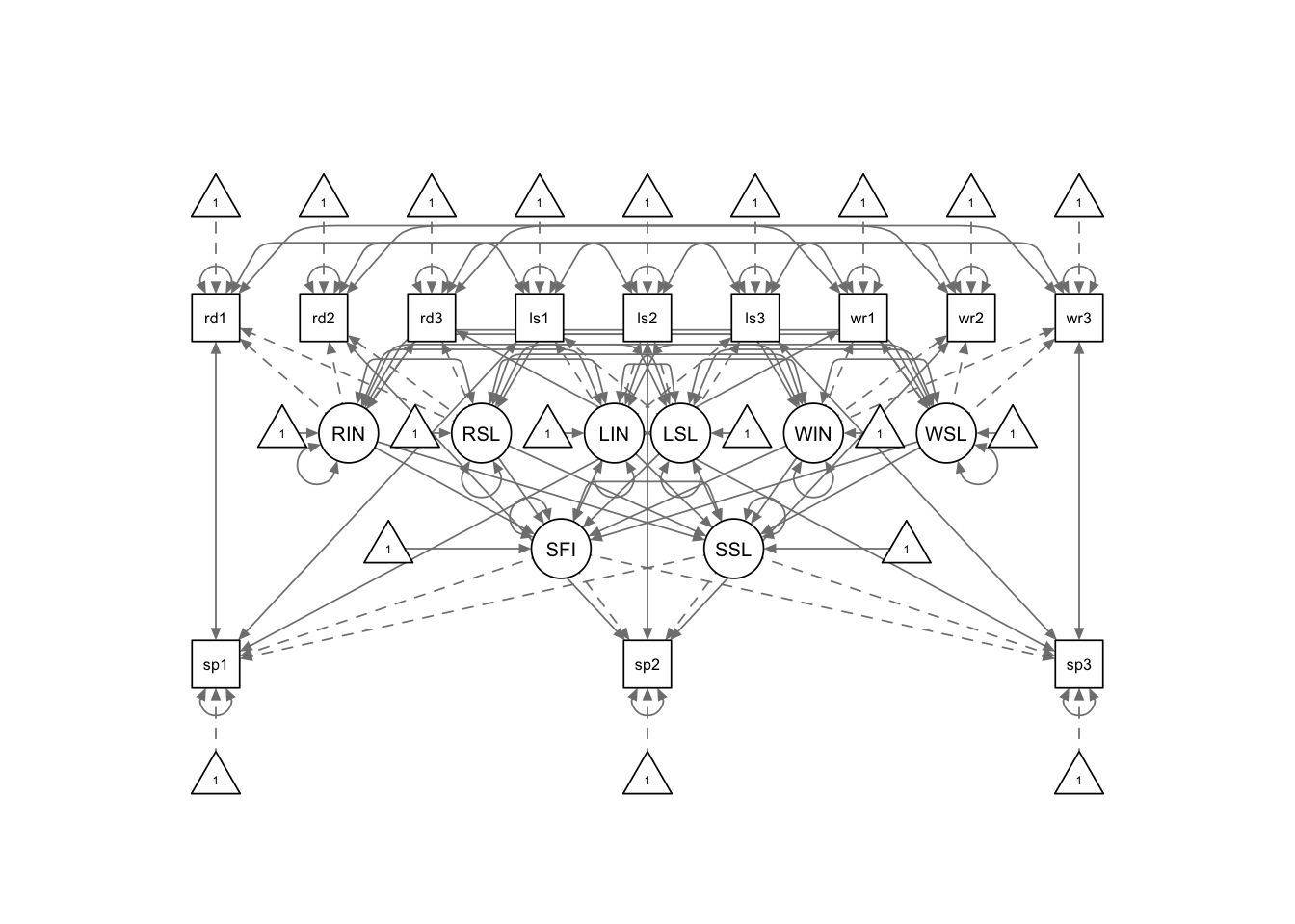
sg.model <- '

RINT =~ 1*read1 + 1*read2 + 1*read3
RSLOPE =~ 0*read1 + 1*read2 + 2*read3

LINT =~ 1*list1 + 1*list2 + 1*list3
LSLOPE =~ 0*list1 + 1*list2 + 2*list3

SFINAL =~ 1*speak1 + 1*speak2 + 1*speak3
SSLOPE =~ -2*speak1 + -1*speak2 + 0*speak3

WINT =~ 1*write1 + 1*write2 + 1*write3
WSLOPE =~ 0*write1 + 1*write2 + 2*write3

RINT ~ 1
RSLOPE ~ 1
LINT ~ 1
LSLOPE ~ 1
SFINAL ~ 1
SSLOPE ~ 1
WINT ~ 1
WSLOPE ~ 1

read1 ~ 0*1
read2 ~ 0*1
read3 ~ 0*1

list1 ~ 0*1
list2 ~ 0*1
list3 ~ 0*1

speak1 ~ 0*1
speak2 ~ 0*1
speak3 ~ 0*1

write1 ~ 0*1
write2 ~ 0*1
write3 ~ 0*1


read1 ~~ list1 + speak1 + write1
read2 ~~ list2 + speak2 + write2
read3 ~~ list3 + speak3 + write3

list1 ~~ speak1 + write1
list2 ~~ speak2 + write2
list3 ~~ speak3 + write3

speak1 ~~ write1
speak2 ~~ write2
speak3 ~~ write3


# structured growth

SFINAL ~ RINT + RSLOPE + LINT + LSLOPE + WINT + WSLOPE
SSLOPE ~ RINT + RSLOPE + LINT + LSLOPE + WINT + WSLOPE

SFINAL ~~ SSLOPE


'

sg.fit <- sem(sg.model, dat)
summary(sg.fit, fit.measures = T)
## lavaan 0.6.15 ended normally after 1028 iterations
##
## Estimator ML
## Optimization method NLMINB
## Number of model parameters 74
##
## Number of observations 170
##
## Model Test User Model:
##
## Test statistic 15.567
## Degrees of freedom 16
## P-value (Chi-square) 0.484
##
## Model Test Baseline Model:
##
## Test statistic 1711.627
## Degrees of freedom 66
## P-value 0.000
##
## User Model versus Baseline Model:
##
## Comparative Fit Index (CFI) 1.000
## Tucker-Lewis Index (TLI) 1.001
##
## Loglikelihood and Information Criteria:
##
## Loglikelihood user model (H0) -5306.076
## Loglikelihood unrestricted model (H1) -5298.293
##
## Akaike (AIC) 10760.153
## Bayesian (BIC) 10992.202
## Sample-size adjusted Bayesian (SABIC) 10757.891
##
## Root Mean Square Error of Approximation:
##
## RMSEA 0.000
## 90 Percent confidence interval - lower 0.000
## 90 Percent confidence interval - upper 0.069
## P-value H_0: RMSEA <= 0.050 0.827
## P-value H_0: RMSEA >= 0.080 0.019
##
## Standardized Root Mean Square Residual:
##
## SRMR 0.029
##
## Parameter Estimates:
##
## Standard errors Standard
## Information Expected
## Information saturated (h1) model Structured
##
## Latent Variables:
## Estimate Std.Err z-value P(>|z|)
## RINT =~
## read1 1.000
## read2 1.000
## read3 1.000
## RSLOPE =~
## read1 0.000
## read2 1.000
## read3 2.000
## LINT =~
## list1 1.000
## list2 1.000
## list3 1.000
## LSLOPE =~
## list1 0.000
## list2 1.000
## list3 2.000
## SFINAL =~
## speak1 1.000
## speak2 1.000
## speak3 1.000
## SSLOPE =~
## speak1 -2.000
## speak2 -1.000
## speak3 0.000
## WINT =~
## write1 1.000
## write2 1.000
## write3 1.000
## WSLOPE =~
## write1 0.000
## write2 1.000
## write3 2.000
##
## Regressions:
## Estimate Std.Err z-value P(>|z|)
## SFINAL ~
## RINT -0.510 0.168 -3.043 0.002
## RSLOPE -0.636 0.945 -0.673 0.501
## LINT 0.456 0.170 2.685 0.007
## LSLOPE 0.878 0.611 1.436 0.151
## WINT 0.740 0.274 2.702 0.007
## WSLOPE 0.040 1.039 0.039 0.969
## SSLOPE ~
## RINT -0.091 0.095 -0.966 0.334
## RSLOPE -0.128 0.618 -0.207 0.836
## LINT 0.034 0.109 0.312 0.755
## LSLOPE 0.286 0.389 0.735 0.463
## WINT 0.037 0.180 0.208 0.835
## WSLOPE -0.280 0.695 -0.403 0.687
##
## Covariances:
## Estimate Std.Err z-value P(>|z|)
## .read1 ~~
## .list1 2.930 2.375 1.234 0.217
## .speak1 0.123 1.424 0.087 0.931
## .write1 -1.807 1.644 -1.100 0.272
## .read2 ~~
## .list2 0.078 1.332 0.059 0.953
## .speak2 -0.147 0.686 -0.214 0.831
## .write2 0.653 0.833 0.784 0.433
## .read3 ~~
## .list3 0.539 2.210 0.244 0.807
## .speak3 0.687 1.228 0.559 0.576
## .write3 -0.698 1.438 -0.486 0.627
## .list1 ~~
## .speak1 0.186 1.443 0.129 0.898
## .write1 2.345 1.608 1.458 0.145
## .list2 ~~
## .speak2 0.432 0.796 0.543 0.587
## .write2 -0.534 0.895 -0.596 0.551
## .list3 ~~
## .speak3 -0.479 1.337 -0.358 0.720
## .write3 0.716 1.483 0.482 0.629
## .speak1 ~~
## .write1 2.183 1.020 2.141 0.032
## .speak2 ~~
## .write2 -0.291 0.484 -0.601 0.548
## .speak3 ~~
## .write3 0.244 0.894 0.273 0.785
## .SFINAL ~~
## .SSLOPE -0.332 0.878 -0.378 0.705
## RINT ~~
## RSLOPE -2.156 1.846 -1.168 0.243
## LINT 17.235 3.569 4.829 0.000
## LSLOPE 1.510 1.540 0.980 0.327
## WINT 17.697 2.602 6.801 0.000
## WSLOPE -1.338 0.998 -1.341 0.180
## RSLOPE ~~
## LINT -0.583 1.458 -0.400 0.689
## LSLOPE 0.645 1.115 0.578 0.563
## WINT -2.329 1.024 -2.275 0.023
## WSLOPE 0.940 0.749 1.255 0.209
## LINT ~~
## LSLOPE -1.869 1.808 -1.034 0.301
## WINT 14.656 2.489 5.888 0.000
## WSLOPE -0.554 0.960 -0.578 0.563
## LSLOPE ~~
## WINT -0.040 1.037 -0.039 0.969
## WSLOPE 0.087 0.748 0.117 0.907
## WINT ~~
## WSLOPE -0.472 0.778 -0.607 0.544
##
## Intercepts:
## Estimate Std.Err z-value P(>|z|)
## RINT 17.383 0.480 36.192 0.000
## RSLOPE 1.091 0.171 6.377 0.000
## LINT 16.626 0.452 36.807 0.000
## LSLOPE 0.984 0.186 5.285 0.000
## .SFINAL 6.504 3.164 2.055 0.040
## .SSLOPE 0.993 2.129 0.467 0.641
## WINT 18.717 0.325 57.663 0.000
## WSLOPE 0.721 0.117 6.186 0.000
## .read1 0.000
## .read2 0.000
## .read3 0.000
## .list1 0.000
## .list2 0.000
## .list3 0.000
## .speak1 0.000
## .speak2 0.000
## .speak3 0.000
## .write1 0.000
## .write2 0.000
## .write3 0.000
##
## Variances:
## Estimate Std.Err z-value P(>|z|)
## .read1 10.733 3.261 3.291 0.001
## .read2 9.325 1.604 5.813 0.000
## .read3 6.482 2.736 2.370 0.018
## .list1 8.924 3.139 2.843 0.004
## .list2 14.574 2.038 7.150 0.000
## .list3 5.193 2.956 1.756 0.079
## .speak1 4.380 1.186 3.694 0.000
## .speak2 2.585 0.563 4.593 0.000
## .speak3 2.404 1.050 2.290 0.022
## .write1 5.482 1.398 3.920 0.000
## .write2 4.196 0.720 5.832 0.000
## .write3 2.963 1.262 2.349 0.019
## RINT 30.800 4.755 6.477 0.000
## RSLOPE 0.790 1.457 0.542 0.588
## LINT 27.172 4.403 6.172 0.000
## LSLOPE 2.468 1.461 1.688 0.091
## .SFINAL 1.895 1.509 1.256 0.209
## .SSLOPE 0.068 0.645 0.106 0.915
## WINT 13.959 2.101 6.645 0.000
## WSLOPE 0.325 0.642 0.506 0.613Example: Second-order LGM
The second-order LGM is discussed in detail in Hancock, Kuo, & Lawrence (2001). In this example, we have data collected from 170 male non-native adult English speakers. Their English language ability has been measured monthly for three months. The data is saved in a txt file named “second_order_data.txt”.
Read the data
setwd(mypath)  # set working directory to where the data file is stored

second.data <- read.delim("second_order_data.txt", sep = '\t', header = F)
colnames(second.data) <- c('read1', 'read2', 'read3', 'list1', 'list2', 'list3',
                        'speak1', 'speak2', 'speak3', 'write1', 'write2', 'write3')

str(second.data)
## 'data.frame': 170 obs. of 12 variables:
## $ read1 : int 22 19 24 21 24 17 14 30 19 11 ...
## $ read2 : int 24 19 26 24 26 21 19 29 23 6 ...
## $ read3 : int 23 17 30 27 28 20 20 29 23 13 ...
## $ list1 : int 28 18 27 18 29 18 14 27 13 15 ...
## $ list2 : int 30 16 30 20 28 16 7 18 10 8 ...
## $ list3 : int 29 17 27 18 26 17 10 24 17 19 ...
## $ speak1: int 23 19 24 22 17 14 14 23 17 23 ...
## $ speak2: int 23 18 24 17 18 17 10 22 17 22 ...
## $ speak3: int 23 18 29 17 19 15 10 23 18 24 ...
## $ write1: int 25 17 21 18 20 21 14 22 17 17 ...
## $ write2: int 22 20 24 21 20 17 18 25 20 18 ...
## $ write3: int 21 25 27 22 22 21 18 22 17 18 ...summary(second.data)## read1 read2 read3 list1
## Min. : 0.00 Min. : 3.00 Min. : 4.00 Min. : 1.00
## 1st Qu.:13.00 1st Qu.:14.00 1st Qu.:16.00 1st Qu.:13.00
## Median :17.00 Median :19.00 Median :20.00 Median :17.00
## Mean :17.38 Mean :18.55 Mean :19.55 Mean :16.56
## 3rd Qu.:22.00 3rd Qu.:23.00 3rd Qu.:23.00 3rd Qu.:21.00
## Max. :30.00 Max. :30.00 Max. :30.00 Max. :30.00
## list2 list3 speak1 speak2
## Min. : 1.00 Min. : 1.00 Min. : 0.00 Min. : 5.00
## 1st Qu.:14.00 1st Qu.:15.00 1st Qu.:15.00 1st Qu.:17.00
## Median :18.00 Median :19.00 Median :18.00 Median :18.00
## Mean :17.63 Mean :18.58 Mean :17.96 Mean :18.73
## 3rd Qu.:21.75 3rd Qu.:23.00 3rd Qu.:20.00 3rd Qu.:22.00
## Max. :30.00 Max. :30.00 Max. :28.00 Max. :27.00
## speak3 write1 write2 write3
## Min. :10.00 Min. : 7.00 Min. : 8.00 Min. : 7.00
## 1st Qu.:17.00 1st Qu.:15.00 1st Qu.:17.00 1st Qu.:18.00
## Median :19.00 Median :20.00 Median :20.00 Median :20.50
## Mean :19.24 Mean :18.59 Mean :19.58 Mean :20.11
## 3rd Qu.:22.00 3rd Qu.:21.00 3rd Qu.:22.00 3rd Qu.:22.00
## Max. :29.00 Max. :30.00 Max. :28.00 Max. :29.00Fit the model
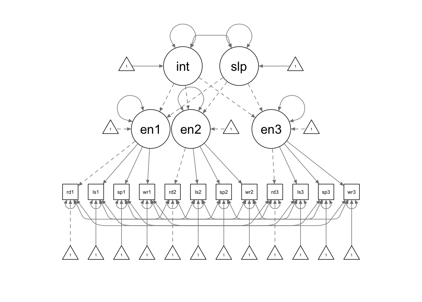
There is still no special syntax required for second-order LGM, although the model syntax looks lengthy. There are a few constraints we need to pay special attention to:
- The item loadings are constrained to be equal across time points (measurement invariance).
- The item whose loading is fixed to 1 also has its intercept fixed to 0.
- The item intercepts are constrained to be equal across time points.
second.model <- '

# first-order latent factors

english1 =~ read1 + a*list1 + b*speak1 + c*write1
english2 =~ read2 + a*list2 + b*speak2 + c*write2
english3 =~ read3 + a*list3 + b*speak3 + c*write3

# second-order growth factors

interc =~ 1*english1 + 1*english2 + 1*english3
slope =~ 0*english1 + 1*english2 + 2*english3

# second-order factor covariances and intercept

interc ~~ slope
interc ~ 1
slope ~ 1

# residual covariances

read1 ~~ read2 + read3
read2 ~~ read3
list1 ~~ list2 + list3
list2 ~~ list3
speak1 ~~ speak2 + speak3
speak2 ~~ speak3
write1 ~~ write2 + write3
write2 ~~ write3

# fix zero intercepts

read1 ~ 0*1
read2 ~ 0*1
read3 ~ 0*1

# equality constraints on the intercepts

list1 ~ d*1
list2 ~ d*1
list3 ~ d*1

speak1 ~ e*1
speak2 ~ e*1
speak3 ~ e*1

write1 ~ f*1
write2 ~ f*1
write3 ~ f*1

'

second.fit <- sem(second.model, second.data)
summary(second.fit, fit.measures = T)
## lavaan 0.6.15 ended normally after 188 iterations
##
## Estimator ML
## Optimization method NLMINB
## Number of model parameters 50
## Number of equality constraints 12
##
## Number of observations 170
##
## Model Test User Model:
##
## Test statistic 109.864
## Degrees of freedom 52
## P-value (Chi-square) 0.000
##
## Model Test Baseline Model:
##
## Test statistic 1711.627
## Degrees of freedom 66
## P-value 0.000
##
## User Model versus Baseline Model:
##
## Comparative Fit Index (CFI) 0.965
## Tucker-Lewis Index (TLI) 0.955
##
## Loglikelihood and Information Criteria:
##
## Loglikelihood user model (H0) -5353.225
## Loglikelihood unrestricted model (H1) -5298.293
##
## Akaike (AIC) 10782.450
## Bayesian (BIC) 10901.610
## Sample-size adjusted Bayesian (SABIC) 10781.289
##
## Root Mean Square Error of Approximation:
##
## RMSEA 0.081
## 90 Percent confidence interval - lower 0.060
## 90 Percent confidence interval - upper 0.102
## P-value H_0: RMSEA <= 0.050 0.010
## P-value H_0: RMSEA >= 0.080 0.548
##
## Standardized Root Mean Square Residual:
##
## SRMR 0.066
##
## Parameter Estimates:
##
## Standard errors Standard
## Information Expected
## Information saturated (h1) model Structured
##
## Latent Variables:
## Estimate Std.Err z-value P(>|z|)
## english1 =~
## read1 1.000
## list1 (a) 1.129 0.096 11.799 0.000
## speak1 (b) 0.657 0.062 10.667 0.000
## write1 (c) 0.835 0.068 12.221 0.000
## english2 =~
## read2 1.000
## list2 (a) 1.129 0.096 11.799 0.000
## speak2 (b) 0.657 0.062 10.667 0.000
## write2 (c) 0.835 0.068 12.221 0.000
## english3 =~
## read3 1.000
## list3 (a) 1.129 0.096 11.799 0.000
## speak3 (b) 0.657 0.062 10.667 0.000
## write3 (c) 0.835 0.068 12.221 0.000
## interc =~
## english1 1.000
## english2 1.000
## english3 1.000
## slope =~
## english1 0.000
## english2 1.000
## english3 2.000
##
## Covariances:
## Estimate Std.Err z-value P(>|z|)
## interc ~~
## slope -0.781 0.732 -1.068 0.286
## .read1 ~~
## .read2 11.998 2.151 5.577 0.000
## .read3 11.178 1.990 5.618 0.000
## .read2 ~~
## .read3 10.096 1.831 5.514 0.000
## .list1 ~~
## .list2 5.659 1.786 3.169 0.002
## .list3 3.769 1.470 2.565 0.010
## .list2 ~~
## .list3 5.682 1.705 3.333 0.001
## .speak1 ~~
## .speak2 4.520 0.800 5.647 0.000
## .speak3 4.329 0.778 5.564 0.000
## .speak2 ~~
## .speak3 4.616 0.763 6.052 0.000
## .write1 ~~
## .write2 1.562 0.741 2.109 0.035
## .write3 1.701 0.702 2.425 0.015
## .write2 ~~
## .write3 2.366 0.744 3.179 0.001
##
## Intercepts:
## Estimate Std.Err z-value P(>|z|)
## interc 17.631 0.450 39.147 0.000
## slope 0.928 0.111 8.337 0.000
## .read1 0.000
## .read2 0.000
## .read3 0.000
## .list1 (d) -3.342 1.837 -1.819 0.069
## .list2 (d) -3.342 1.837 -1.819 0.069
## .list3 (d) -3.342 1.837 -1.819 0.069
## .speak1 (e) 6.455 1.186 5.441 0.000
## .speak2 (e) 6.455 1.186 5.441 0.000
## .speak3 (e) 6.455 1.186 5.441 0.000
## .write1 (f) 3.934 1.310 3.002 0.003
## .write2 (f) 3.934 1.310 3.002 0.003
## .write3 (f) 3.934 1.310 3.002 0.003
## .english1 0.000
## .english2 0.000
## .english3 0.000
##
## Variances:
## Estimate Std.Err z-value P(>|z|)
## .read1 23.986 2.918 8.220 0.000
## .list1 14.093 2.060 6.841 0.000
## .speak1 8.241 1.037 7.945 0.000
## .write1 5.534 0.944 5.864 0.000
## .read2 19.614 2.384 8.228 0.000
## .list2 20.410 2.607 7.830 0.000
## .speak2 7.290 0.904 8.064 0.000
## .write2 6.399 0.960 6.668 0.000
## .read3 16.424 2.059 7.978 0.000
## .list3 12.798 1.821 7.029 0.000
## .speak3 7.018 0.880 7.971 0.000
## .write3 5.524 0.870 6.346 0.000
## .english1 1.501 1.340 1.120 0.263
## .english2 -0.106 0.635 -0.167 0.868
## .english3 0.320 1.199 0.267 0.790
## interc 17.577 3.307 5.314 0.000
## slope 0.304 0.623 0.488 0.625Example: Shifting Indicators
Note that we can use the NA label to free the first
loading.
si.model <- '

# first-order latent factors

english1 =~ read1 + a*list1
english2 =~ NA*list2 + a*list2 + b*speak2
english3 =~ NA*speak3 + b*speak3 + write3

# second-order growth factors

interc =~ 1*english1 + 1*english2 + 1*english3
slope =~ 0*english1 + 1*english2 + 2*english3

# second-order factor covariances and intercept

interc ~~ slope
interc ~ 1
slope ~ 1

# residual covariances
list1 ~~ list2
speak2 ~~ speak3

# fix zero intercepts
read1 ~ 0*1

# equality constraints on the intercepts

list1 ~ d*1
list2 ~ d*1

speak2 ~ e*1
speak3 ~ e*1

write3 ~ 1

'

si.fit <- sem(si.model, second.data)
summary(si.fit, fit.measures = T)
## lavaan 0.6.15 ended normally after 157 iterations
##
## Estimator ML
## Optimization method NLMINB
## Number of model parameters 26
## Number of equality constraints 4
##
## Number of observations 170
##
## Model Test User Model:
##
## Test statistic 25.370
## Degrees of freedom 5
## P-value (Chi-square) 0.000
##
## Model Test Baseline Model:
##
## Test statistic 582.446
## Degrees of freedom 15
## P-value 0.000
##
## User Model versus Baseline Model:
##
## Comparative Fit Index (CFI) 0.964
## Tucker-Lewis Index (TLI) 0.892
##
## Loglikelihood and Information Criteria:
##
## Loglikelihood user model (H0) -2794.776
## Loglikelihood unrestricted model (H1) -2782.091
##
## Akaike (AIC) 5633.551
## Bayesian (BIC) 5702.539
## Sample-size adjusted Bayesian (SABIC) 5632.879
##
## Root Mean Square Error of Approximation:
##
## RMSEA 0.155
## 90 Percent confidence interval - lower 0.098
## 90 Percent confidence interval - upper 0.217
## P-value H_0: RMSEA <= 0.050 0.002
## P-value H_0: RMSEA >= 0.080 0.983
##
## Standardized Root Mean Square Residual:
##
## SRMR 0.040
##
## Parameter Estimates:
##
## Standard errors Standard
## Information Expected
## Information saturated (h1) model Structured
##
## Latent Variables:
## Estimate Std.Err z-value P(>|z|)
## english1 =~
## read1 1.000
## list1 (a) 1.250 0.167 7.466 0.000
## english2 =~
## list2 (a) 1.250 0.167 7.466 0.000
## speak2 (b) 0.852 0.138 6.164 0.000
## english3 =~
## speak3 (b) 0.852 0.138 6.164 0.000
## write3 1.039 0.182 5.696 0.000
## interc =~
## english1 1.000
## english2 1.000
## english3 1.000
## slope =~
## english1 0.000
## english2 1.000
## english3 2.000
##
## Covariances:
## Estimate Std.Err z-value P(>|z|)
## interc ~~
## slope -1.271 0.979 -1.298 0.194
## .list1 ~~
## .list2 5.139 1.966 2.614 0.009
## .speak2 ~~
## .speak3 3.482 0.815 4.271 0.000
##
## Intercepts:
## Estimate Std.Err z-value P(>|z|)
## interc 17.397 0.491 35.416 0.000
## slope 0.678 0.197 3.441 0.001
## .read1 0.000
## .list1 (d) -5.096 2.964 -1.719 0.086
## .list2 (d) -5.096 2.964 -1.719 0.086
## .speak2 (e) 3.296 2.463 1.339 0.181
## .speak3 (e) 3.296 2.463 1.339 0.181
## .write3 0.606 3.311 0.183 0.855
## .english1 0.000
## .english2 0.000
## .english3 0.000
##
## Variances:
## Estimate Std.Err z-value P(>|z|)
## .read1 25.033 3.186 7.857 0.000
## .list1 11.701 2.778 4.212 0.000
## .list2 19.766 2.763 7.154 0.000
## .speak2 5.809 0.976 5.951 0.000
## .speak3 6.226 0.893 6.973 0.000
## .write3 5.955 1.090 5.465 0.000
## .english1 1.989 2.136 0.931 0.352
## .english2 0.628 0.997 0.630 0.529
## .english3 -0.814 1.506 -0.540 0.589
## interc 14.155 4.020 3.521 0.000
## slope 0.432 0.779 0.555 0.579Example: LGM with ordinal data
Assume we want to fit a linear LGM with ordinal data collected at four equally spaced time points. The data is saved in a txt file named “categorical_data.txt” in your course materials.
Read the data
setwd(mypath)  # set working directory to where the data file is stored

cat.data <- read.table("categorical_data.txt", header = F)
colnames(cat.data) <- c("y1", "y2", "y3", "y4")

cat.data <- apply(cat.data, 2, ordered)

str(cat.data)
## chr [1:369, 1:4] "0" "0" "1" "0" "0" "0" "0" "0" "0" "0" "0" "0" "0" ...
## - attr(*, "dimnames")=List of 2
## ..$ : NULL
## ..$ : chr [1:4] "y1" "y2" "y3" "y4"summary(cat.data)## y1 y2 y3
## Length:369 Length:369 Length:369
## Class :character Class :character Class :character
## Mode :character Mode :character Mode :character
## y4
## Length:369
## Class :character
## Mode :characterFit the model
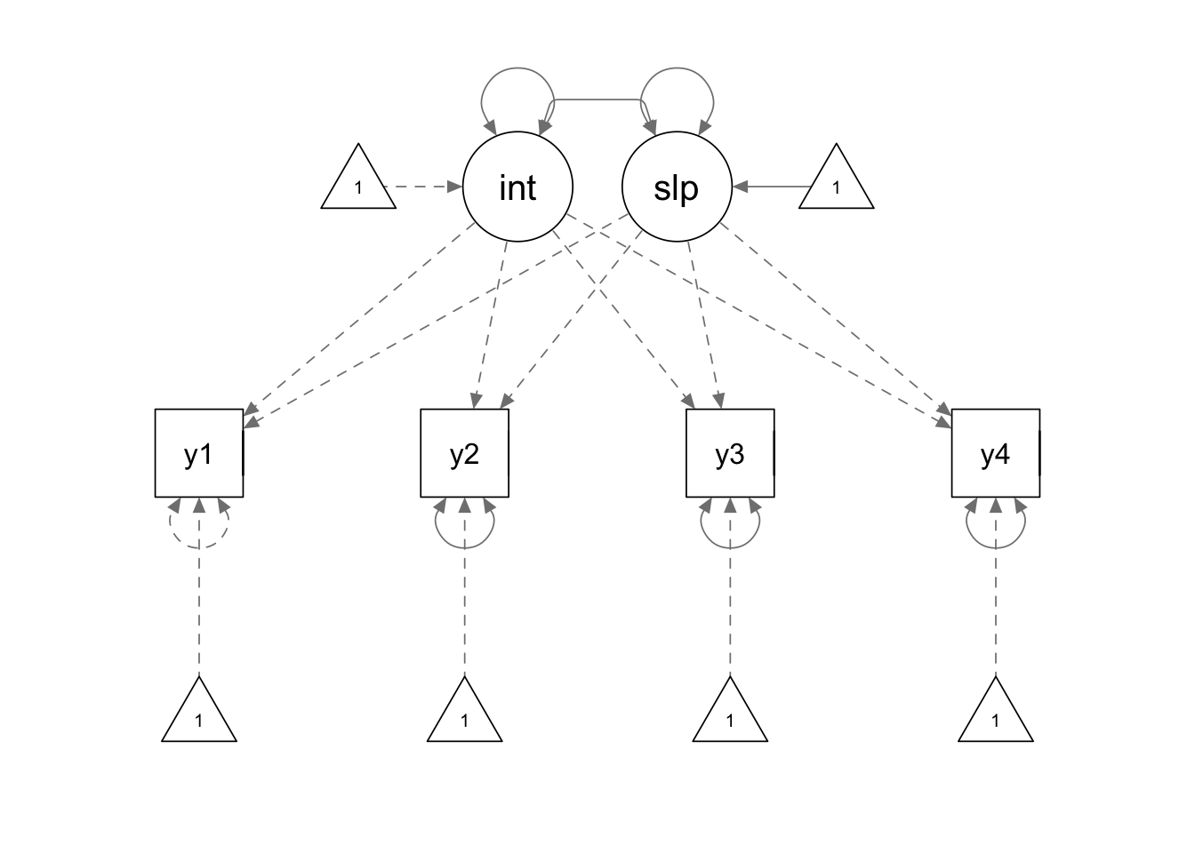
We define our model using the following model syntax. Some notes for this model syntax:
- We fix the latent intercept mean to be zero;
- We use the “|” operator to define the thresholds of the endogenous categorical variables: y1-y4. The thresholds are named “t1” and “t2” by convention and they are listed on the right side of the formulas. We give them parameter labels to impose the equality constraints.
When calling up the fitting function, we use the
ordered = argument to specify the categorical variables. We
can also request theta parameterization using the
parameterization = argument.
cat.lgm <- '

# growth latent factors

interc =~ 1*y1 + 1*y2 + 1*y3 + 1*y4
slope =~ 0*y1 + 1*y2 + 2*y3 + 3*y4


# means of latent factors

interc ~ 0*1
slope ~ 1


# Equality constraints on the threshold
y1 | a*t1 + b*t2
y2 | a*t1 + b*t2
y3 | a*t1 + b*t2
y4 | a*t1 + b*t2


# variances

y1 ~~ 1*y1
y2 ~~ y2
y3 ~~ y3
y4 ~~ y4

'

cat.fit <- sem(cat.lgm, cat.data, ordered = c("y1","y2","y3","y4"), parameterization = "theta")

summary(cat.fit, fit.measures = T)
## lavaan 0.6.15 ended normally after 61 iterations
##
## Estimator DWLS
## Optimization method NLMINB
## Number of model parameters 15
## Number of equality constraints 6
##
## Number of observations 369
##
## Model Test User Model:
## Standard Scaled
## Test Statistic 2.355 4.948
## Degrees of freedom 5 5
## P-value (Chi-square) 0.798 0.422
## Scaling correction factor 0.530
## Shift parameter 0.507
## simple second-order correction
##
## Model Test Baseline Model:
##
## Test statistic 680.838 502.371
## Degrees of freedom 6 6
## P-value 0.000 0.000
## Scaling correction factor 1.360
##
## User Model versus Baseline Model:
##
## Comparative Fit Index (CFI) 1.000 1.000
## Tucker-Lewis Index (TLI) 1.005 1.000
##
## Robust Comparative Fit Index (CFI) NA
## Robust Tucker-Lewis Index (TLI) NA
##
## Root Mean Square Error of Approximation:
##
## RMSEA 0.000 0.000
## 90 Percent confidence interval - lower 0.000 0.000
## 90 Percent confidence interval - upper 0.046 0.072
## P-value H_0: RMSEA <= 0.050 0.961 0.806
## P-value H_0: RMSEA >= 0.080 0.003 0.026
##
## Robust RMSEA NA
## 90 Percent confidence interval - lower NA
## 90 Percent confidence interval - upper NA
## P-value H_0: Robust RMSEA <= 0.050 NA
## P-value H_0: Robust RMSEA >= 0.080 NA
##
## Standardized Root Mean Square Residual:
##
## SRMR 0.033 0.033
##
## Parameter Estimates:
##
## Standard errors Robust.sem
## Information Expected
## Information saturated (h1) model Unstructured
##
## Latent Variables:
## Estimate Std.Err z-value P(>|z|)
## interc =~
## y1 1.000
## y2 1.000
## y3 1.000
## y4 1.000
## slope =~
## y1 0.000
## y2 1.000
## y3 2.000
## y4 3.000
##
## Covariances:
## Estimate Std.Err z-value P(>|z|)
## interc ~~
## slope -0.311 0.301 -1.031 0.302
##
## Intercepts:
## Estimate Std.Err z-value P(>|z|)
## interc 0.000
## slope 0.441 0.199 2.214 0.027
## .y1 0.000
## .y2 0.000
## .y3 0.000
## .y4 0.000
##
## Thresholds:
## Estimate Std.Err z-value P(>|z|)
## y1|t1 (a) 3.028 0.587 5.160 0.000
## y1|t2 (b) 3.773 0.695 5.428 0.000
## y2|t1 (a) 3.028 0.587 5.160 0.000
## y2|t2 (b) 3.773 0.695 5.428 0.000
## y3|t1 (a) 3.028 0.587 5.160 0.000
## y3|t2 (b) 3.773 0.695 5.428 0.000
## y4|t1 (a) 3.028 0.587 5.160 0.000
## y4|t2 (b) 3.773 0.695 5.428 0.000
##
## Variances:
## Estimate Std.Err z-value P(>|z|)
## .y1 1.000
## .y2 0.511 0.257 1.994 0.046
## .y3 0.804 0.405 1.987 0.047
## .y4 0.574 0.382 1.502 0.133
## interc 2.941 1.382 2.128 0.033
## slope 0.090 0.096 0.935 0.350
##
## Scales y*:
## Estimate Std.Err z-value P(>|z|)
## y1 0.504
## y2 0.585
## y3 0.591
## y4 0.638Example: LGM with distal categorical outcome
Read the data
setwd(mypath)  # set working directory to where the data file is stored

dat <- read.table("distal_data.csv", sep = ",", header = F)
colnames(dat) <- c(paste0("math", 7:10), "dropout")

dat$dropout <- ordered(dat$dropout)

str(dat)
## 'data.frame': 1994 obs. of 5 variables:
## $ math7 : num 62 61.2 59.4 54.6 62 ...
## $ math8 : num 62.3 60.3 54.8 51.2 61 ...
## $ math9 : num 69 64.4 59.4 64.1 62.4 ...
## $ math10 : num 68.4 65.3 63 62.3 61.5 ...
## $ dropout: Ord.factor w/ 2 levels "0"<"1": 1 1 1 1 1 1 1 1 1 2 ...summary(dat)## math7 math8 math9 math10 dropout
## Min. :28.19 Min. :23.85 Min. :28.61 Min. :28.16 0:1608
## 1st Qu.:45.49 1st Qu.:48.42 1st Qu.:51.08 1st Qu.:53.29 1: 386
## Median :53.15 Median :55.75 Median :59.31 Median :62.88
## Mean :52.20 Mean :54.80 Mean :58.60 Mean :61.42
## 3rd Qu.:59.62 3rd Qu.:61.79 3rd Qu.:66.77 3rd Qu.:69.95
## Max. :83.97 Max. :84.17 Max. :88.88 Max. :93.96Fit the model
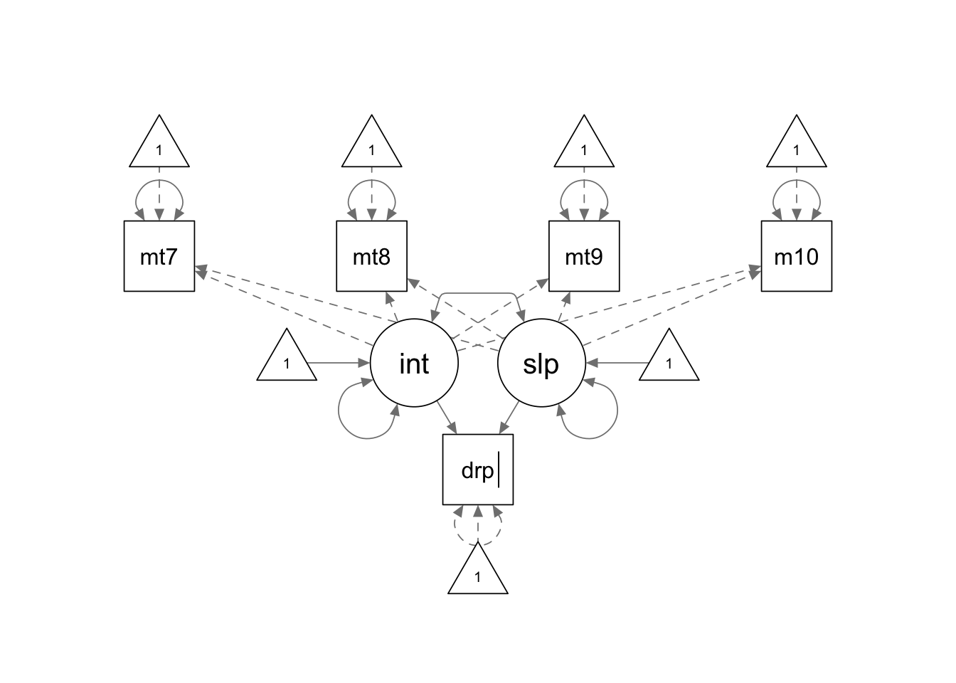
distal.model <- '

interc =~ 1*math7 + 1*math8 + 1*math9 + 1*math10
slope =~ 0*math7 + 1*math8 + 2*math9 + 3*math10

interc ~ 1
slope ~ 1

math7 ~ 0*1
math8 ~ 0*1
math9 ~ 0*1
math10 ~ 0*1

dropout ~ interc + slope

'

distal.fit <- sem(distal.model, dat, ordered = c("dropout"), parameterization = "delta")

summary(distal.fit, fit.measures = T)
## lavaan 0.6.15 ended normally after 104 iterations
##
## Estimator DWLS
## Optimization method NLMINB
## Number of model parameters 12
##
## Number of observations 1994
##
## Model Test User Model:
## Standard Scaled
## Test Statistic 5.459 37.170
## Degrees of freedom 7 7
## P-value (Chi-square) 0.604 0.000
## Scaling correction factor 0.149
## Shift parameter 0.597
## simple second-order correction
##
## Model Test Baseline Model:
##
## Test statistic 3977.646 1996.833
## Degrees of freedom 10 10
## P-value 0.000 0.000
## Scaling correction factor 1.997
##
## User Model versus Baseline Model:
##
## Comparative Fit Index (CFI) 1.000 0.985
## Tucker-Lewis Index (TLI) 1.001 0.978
##
## Robust Comparative Fit Index (CFI) NA
## Robust Tucker-Lewis Index (TLI) NA
##
## Root Mean Square Error of Approximation:
##
## RMSEA 0.000 0.047
## 90 Percent confidence interval - lower 0.000 0.032
## 90 Percent confidence interval - upper 0.024 0.062
## P-value H_0: RMSEA <= 0.050 1.000 0.622
## P-value H_0: RMSEA >= 0.080 0.000 0.000
##
## Robust RMSEA NA
## 90 Percent confidence interval - lower NA
## 90 Percent confidence interval - upper NA
## P-value H_0: Robust RMSEA <= 0.050 NA
## P-value H_0: Robust RMSEA >= 0.080 NA
##
## Standardized Root Mean Square Residual:
##
## SRMR 0.008 0.008
##
## Parameter Estimates:
##
## Standard errors Robust.sem
## Information Expected
## Information saturated (h1) model Unstructured
##
## Latent Variables:
## Estimate Std.Err z-value P(>|z|)
## interc =~
## math7 1.000
## math8 1.000
## math9 1.000
## math10 1.000
## slope =~
## math7 0.000
## math8 1.000
## math9 2.000
## math10 3.000
##
## Regressions:
## Estimate Std.Err z-value P(>|z|)
## dropout ~
## interc 0.002 0.006 0.273 0.785
## slope -0.040 0.049 -0.816 0.414
##
## Covariances:
## Estimate Std.Err z-value P(>|z|)
## interc ~~
## slope 4.850 0.881 5.505 0.000
##
## Intercepts:
## Estimate Std.Err z-value P(>|z|)
## interc 52.042 0.211 246.670 0.000
## slope 3.139 0.062 50.970 0.000
## .math7 0.000
## .math8 0.000
## .math9 0.000
## .math10 0.000
## .dropout 0.000
##
## Thresholds:
## Estimate Std.Err z-value P(>|z|)
## dropout|t1 0.819 0.212 3.868 0.000
##
## Variances:
## Estimate Std.Err z-value P(>|z|)
## .math7 17.257 2.006 8.604 0.000
## .math8 12.314 1.552 7.936 0.000
## .math9 20.216 1.995 10.135 0.000
## .math10 36.533 3.006 12.152 0.000
## .dropout 0.997
## interc 76.279 3.175 24.028 0.000
## slope 2.168 0.420 5.156 0.000
##
## Scales y*:
## Estimate Std.Err z-value P(>|z|)
## dropout 1.000Example: Latent Change Score Models
Read the data
setwd(mypath)  # set working directory to where the data file is stored

dat <- read.table("Read-Data-Mplus.dat", sep = "\t", header = F, na.strings = "-99")

colnames(dat) <-c('id', 'gen', 'momage', 'homecog', 'homeemo', paste0('an', 1:4), paste0('r', 1:4), paste0('ag', 1:4))

str(dat)
## 'data.frame': 405 obs. of 17 variables:
## $ id : int 1 2 3 4 5 6 7 8 9 10 ...
## $ gen : int 1 1 0 1 1 0 0 0 0 0 ...
## $ momage : int 27 27 27 24 26 25 22 23 24 28 ...
## $ homecog: int 7 10 7 8 8 6 5 1 3 9 ...
## $ homeemo: int 11 7 7 8 8 11 5 4 7 11 ...
## $ an1 : int 1 1 5 1 2 1 3 0 5 2 ...
## $ an2 : int 0 1 0 1 3 0 NA NA 3 3 ...
## $ an3 : int 1 0 5 NA 3 0 0 0 2 6 ...
## $ an4 : int 0 1 3 NA 1 0 10 4 0 5 ...
## $ r1 : int 27 31 36 18 23 21 21 13 29 45 ...
## $ r2 : int 49 47 52 30 49 NA NA NA NA 58 ...
## $ r3 : int 50 56 60 NA NA 45 48 37 35 76 ...
## $ r4 : int NA 64 75 NA 77 53 NA NA 38 80 ...
## $ ag1 : int 6 7 8 7 6 6 7 6 8 8 ...
## $ ag2 : int 9 10 11 10 9 9 NA NA 10 10 ...
## $ ag3 : int 11 12 13 NA 11 11 11 10 12 12 ...
## $ ag4 : int 13 14 14 NA 13 13 13 12 14 15 ...summary(dat)## id gen momage homecog
## Min. : 1 Min. :0.0000 Min. :21.00 Min. : 1.000
## 1st Qu.:102 1st Qu.:0.0000 1st Qu.:24.00 1st Qu.: 7.000
## Median :203 Median :1.0000 Median :26.00 Median : 9.000
## Mean :203 Mean :0.5012 Mean :25.53 Mean : 8.894
## 3rd Qu.:304 3rd Qu.:1.0000 3rd Qu.:27.00 3rd Qu.:11.000
## Max. :405 Max. :1.0000 Max. :29.00 Max. :14.000
##
## homeemo an1 an2 an3
## Min. : 0.000 Min. :0.000 Min. : 0.000 Min. : 0.000
## 1st Qu.: 8.000 1st Qu.:0.000 1st Qu.: 0.000 1st Qu.: 0.000
## Median :10.000 Median :1.000 Median : 1.500 Median : 1.000
## Mean : 9.205 Mean :1.662 Mean : 2.027 Mean : 1.828
## 3rd Qu.:11.000 3rd Qu.:3.000 3rd Qu.: 3.000 3rd Qu.: 3.000
## Max. :13.000 Max. :9.000 Max. :10.000 Max. :10.000
## NA's :31 NA's :108
## an4 r1 r2 r3
## Min. : 0.000 Min. : 1.00 Min. :16.00 Min. :22.00
## 1st Qu.: 0.000 1st Qu.:18.00 1st Qu.:33.00 1st Qu.:42.00
## Median : 1.500 Median :23.00 Median :41.00 Median :50.00
## Mean : 2.061 Mean :25.23 Mean :40.76 Mean :50.05
## 3rd Qu.: 3.000 3rd Qu.:30.00 3rd Qu.:49.00 3rd Qu.:58.00
## Max. :10.000 Max. :72.00 Max. :82.00 Max. :84.00
## NA's :111 NA's :30 NA's :130
## r4 ag1 ag2 ag3
## Min. :25.00 Min. :6.000 Min. : 8.000 Min. :10.00
## 1st Qu.:49.25 1st Qu.:6.000 1st Qu.: 9.000 1st Qu.:11.00
## Median :58.00 Median :7.000 Median : 9.000 Median :11.00
## Mean :57.74 Mean :6.983 Mean : 9.353 Mean :11.43
## 3rd Qu.:66.75 3rd Qu.:8.000 3rd Qu.:10.000 3rd Qu.:12.00
## Max. :83.00 Max. :8.000 Max. :11.000 Max. :13.00
## NA's :135 NA's :31 NA's :108
## ag4
## Min. :12.0
## 1st Qu.:13.0
## Median :13.0
## Mean :13.3
## 3rd Qu.:14.0
## Max. :15.0
## NA's :111Constant Change
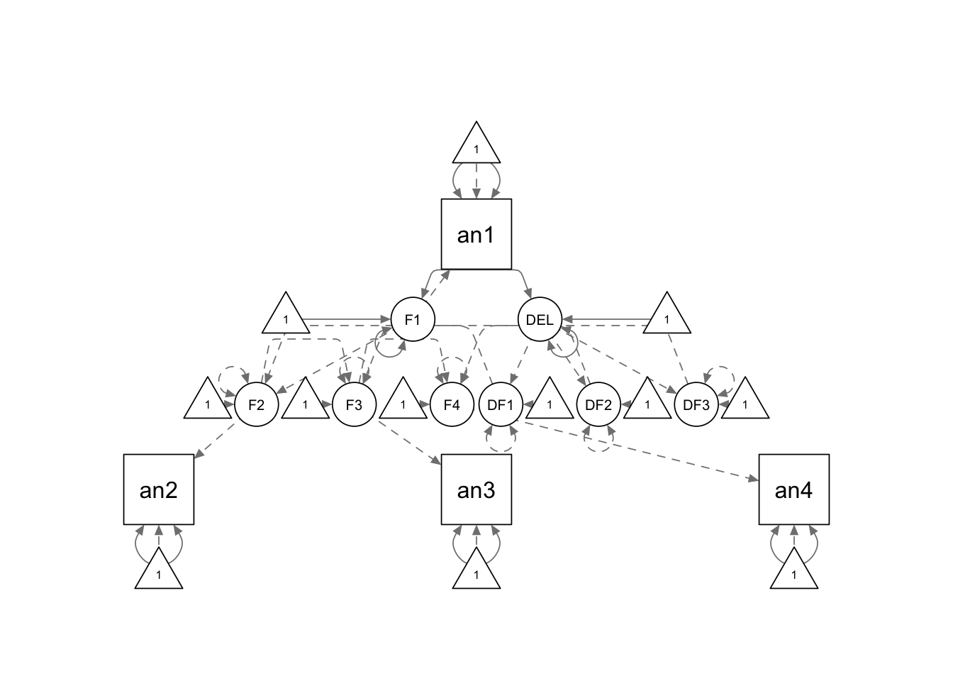
cc.model <- '

F1 =~ an1
F2 =~ an2
F3 =~ an3
F4 =~ an4

# error variance
an1 ~~ theta*an1
an2 ~~ theta*an2
an3 ~~ theta*an3
an4 ~~ theta*an4


DF12 =~ 1*F2
DF23 =~ 1*F3
DF34 =~ 1*F4

# constant latent change
DELTA =~ 1*DF12 + 1*DF23 + 1*DF34

F1 ~~ F1
DELTA ~~ DELTA

F2 ~~ 0*F2
F3 ~~ 0*F3
F4 ~~ 0*F4

DF12 ~~ 0*DF12
DF23 ~~ 0*DF23
DF34 ~~ 0*DF34

F1 ~~ DELTA

F2 ~ 1*F1
F3 ~ 1*F2
F4 ~ 1*F3

F1 ~ 1
DELTA ~ 1

F2 ~ 0*1
F3 ~ 0*1
F4 ~ 0*1

DF12 ~ 0*1
DF23 ~ 0*1
DF34 ~ 0*1

an1 ~ 0*1
an2 ~ 0*1
an3 ~ 0*1
an4 ~ 0*1

'

cc.fit <- sem(cc.model, dat, estimator = "MLR", missing = "fiml")


summary(cc.fit, fit.measures = T)
## lavaan 0.6.15 ended normally after 18 iterations
##
## Estimator ML
## Optimization method NLMINB
## Number of model parameters 9
## Number of equality constraints 3
##
## Number of observations 405
## Number of missing patterns 8
##
## Model Test User Model:
## Standard Scaled
## Test Statistic 19.923 14.891
## Degrees of freedom 8 8
## P-value (Chi-square) 0.011 0.061
## Scaling correction factor 1.338
## Yuan-Bentler correction (Mplus variant)
##
## Model Test Baseline Model:
##
## Test statistic 366.752 254.284
## Degrees of freedom 6 6
## P-value 0.000 0.000
## Scaling correction factor 1.442
##
## User Model versus Baseline Model:
##
## Comparative Fit Index (CFI) 0.967 0.972
## Tucker-Lewis Index (TLI) 0.975 0.979
##
## Robust Comparative Fit Index (CFI) 0.984
## Robust Tucker-Lewis Index (TLI) 0.988
##
## Loglikelihood and Information Criteria:
##
## Loglikelihood user model (H0) -2655.038 -2655.038
## Scaling correction factor 0.956
## for the MLR correction
## Loglikelihood unrestricted model (H1) -2645.076 -2645.076
## Scaling correction factor 1.379
## for the MLR correction
##
## Akaike (AIC) 5322.075 5322.075
## Bayesian (BIC) 5346.098 5346.098
## Sample-size adjusted Bayesian (SABIC) 5327.060 5327.060
##
## Root Mean Square Error of Approximation:
##
## RMSEA 0.061 0.046
## 90 Percent confidence interval - lower 0.027 0.009
## 90 Percent confidence interval - upper 0.095 0.077
## P-value H_0: RMSEA <= 0.050 0.261 0.537
## P-value H_0: RMSEA >= 0.080 0.192 0.035
##
## Robust RMSEA 0.051
## 90 Percent confidence interval - lower 0.000
## 90 Percent confidence interval - upper 0.103
## P-value H_0: Robust RMSEA <= 0.050 0.427
## P-value H_0: Robust RMSEA >= 0.080 0.210
##
## Standardized Root Mean Square Residual:
##
## SRMR 0.074 0.074
##
## Parameter Estimates:
##
## Standard errors Sandwich
## Information bread Observed
## Observed information based on Hessian
##
## Latent Variables:
## Estimate Std.Err z-value P(>|z|)
## F1 =~
## an1 1.000
## F2 =~
## an2 1.000
## F3 =~
## an3 1.000
## F4 =~
## an4 1.000
## DF12 =~
## F2 1.000
## DF23 =~
## F3 1.000
## DF34 =~
## F4 1.000
## DELTA =~
## DF12 1.000
## DF23 1.000
## DF34 1.000
##
## Regressions:
## Estimate Std.Err z-value P(>|z|)
## F2 ~
## F1 1.000
## F3 ~
## F2 1.000
## F4 ~
## F3 1.000
##
## Covariances:
## Estimate Std.Err z-value P(>|z|)
## F1 ~~
## DELTA 0.196 0.082 2.383 0.017
##
## Intercepts:
## Estimate Std.Err z-value P(>|z|)
## F1 1.715 0.079 21.758 0.000
## DELTA 0.151 0.039 3.845 0.000
## .F2 0.000
## .F3 0.000
## .F4 0.000
## .DF12 0.000
## .DF23 0.000
## .DF34 0.000
## .an1 0.000
## .an2 0.000
## .an3 0.000
## .an4 0.000
##
## Variances:
## Estimate Std.Err z-value P(>|z|)
## .an1 (thet) 1.740 0.146 11.882 0.000
## .an2 (thet) 1.740 0.146 11.882 0.000
## .an3 (thet) 1.740 0.146 11.882 0.000
## .an4 (thet) 1.740 0.146 11.882 0.000
## F1 1.242 0.242 5.144 0.000
## DELTA 0.103 0.052 2.002 0.045
## .F2 0.000
## .F3 0.000
## .F4 0.000
## .DF12 0.000
## .DF23 0.000
## .DF34 0.000Dual Change
dc.model <- '

F1 =~ an1
F2 =~ an2
F3 =~ an3
F4 =~ an4

# error variance
an1 ~~ theta*an1
an2 ~~ theta*an2
an3 ~~ theta*an3
an4 ~~ theta*an4

# dual change
DF12 =~ 1*F2
DF23 =~ 1*F3
DF34 =~ 1*F4

DF12 ~ b*F1
DF23 ~ b*F2
DF34 ~ b*F3

DELTA =~ 1*DF12 + 1*DF23 + 1*DF34

F1 ~~ F1
DELTA ~~ DELTA

F2 ~~ 0*F2
F3 ~~ 0*F3
F4 ~~ 0*F4

DF12 ~~ 0*DF12
DF23 ~~ 0*DF23
DF34 ~~ 0*DF34

F1 ~~ DELTA

F2 ~ 1*F1
F3 ~ 1*F2
F4 ~ 1*F3

F1 ~ 1
DELTA ~ 1

F2 ~ 0*1
F3 ~ 0*1
F4 ~ 0*1

DF12 ~ 0*1
DF23 ~ 0*1
DF34 ~ 0*1

an1 ~ 0*1
an2 ~ 0*1
an3 ~ 0*1
an4 ~ 0*1

'

dc.fit <- sem(dc.model, dat, estimator = "MLR", missing = "fiml")


summary(dc.fit, fit.measures = T)
## lavaan 0.6.15 ended normally after 35 iterations
##
## Estimator ML
## Optimization method NLMINB
## Number of model parameters 12
## Number of equality constraints 5
##
## Number of observations 405
## Number of missing patterns 8
##
## Model Test User Model:
## Standard Scaled
## Test Statistic 12.181 11.959
## Degrees of freedom 7 7
## P-value (Chi-square) 0.095 0.102
## Scaling correction factor 1.019
## Yuan-Bentler correction (Mplus variant)
##
## Model Test Baseline Model:
##
## Test statistic 366.752 254.284
## Degrees of freedom 6 6
## P-value 0.000 0.000
## Scaling correction factor 1.442
##
## User Model versus Baseline Model:
##
## Comparative Fit Index (CFI) 0.986 0.980
## Tucker-Lewis Index (TLI) 0.988 0.983
##
## Robust Comparative Fit Index (CFI) 0.989
## Robust Tucker-Lewis Index (TLI) 0.991
##
## Loglikelihood and Information Criteria:
##
## Loglikelihood user model (H0) -2651.166 -2651.166
## Scaling correction factor 1.015
## for the MLR correction
## Loglikelihood unrestricted model (H1) -2645.076 -2645.076
## Scaling correction factor 1.379
## for the MLR correction
##
## Akaike (AIC) 5316.333 5316.333
## Bayesian (BIC) 5344.360 5344.360
## Sample-size adjusted Bayesian (SABIC) 5322.148 5322.148
##
## Root Mean Square Error of Approximation:
##
## RMSEA 0.043 0.042
## 90 Percent confidence interval - lower 0.000 0.000
## 90 Percent confidence interval - upper 0.082 0.081
## P-value H_0: RMSEA <= 0.050 0.565 0.581
## P-value H_0: RMSEA >= 0.080 0.060 0.054
##
## Robust RMSEA 0.044
## 90 Percent confidence interval - lower 0.000
## 90 Percent confidence interval - upper 0.101
## P-value H_0: Robust RMSEA <= 0.050 0.499
## P-value H_0: Robust RMSEA >= 0.080 0.174
##
## Standardized Root Mean Square Residual:
##
## SRMR 0.062 0.062
##
## Parameter Estimates:
##
## Standard errors Sandwich
## Information bread Observed
## Observed information based on Hessian
##
## Latent Variables:
## Estimate Std.Err z-value P(>|z|)
## F1 =~
## an1 1.000
## F2 =~
## an2 1.000
## F3 =~
## an3 1.000
## F4 =~
## an4 1.000
## DF12 =~
## F2 1.000
## DF23 =~
## F3 1.000
## DF34 =~
## F4 1.000
## DELTA =~
## DF12 1.000
## DF23 1.000
## DF34 1.000
##
## Regressions:
## Estimate Std.Err z-value P(>|z|)
## DF12 ~
## F1 (b) -0.670 0.337 -1.988 0.047
## DF23 ~
## F2 (b) -0.670 0.337 -1.988 0.047
## DF34 ~
## F3 (b) -0.670 0.337 -1.988 0.047
## F2 ~
## F1 1.000
## F3 ~
## F2 1.000
## F4 ~
## F3 1.000
##
## Covariances:
## Estimate Std.Err z-value P(>|z|)
## F1 ~~
## DELTA 1.050 0.450 2.336 0.019
##
## Intercepts:
## Estimate Std.Err z-value P(>|z|)
## F1 1.665 0.082 20.233 0.000
## DELTA 1.406 0.635 2.213 0.027
## .F2 0.000
## .F3 0.000
## .F4 0.000
## .DF12 0.000
## .DF23 0.000
## .DF34 0.000
## .an1 0.000
## .an2 0.000
## .an3 0.000
## .an4 0.000
##
## Variances:
## Estimate Std.Err z-value P(>|z|)
## .an1 (thet) 1.720 0.160 10.736 0.000
## .an2 (thet) 1.720 0.160 10.736 0.000
## .an3 (thet) 1.720 0.160 10.736 0.000
## .an4 (thet) 1.720 0.160 10.736 0.000
## F1 1.068 0.297 3.600 0.000
## DELTA 1.337 1.039 1.287 0.198
## .F2 0.000
## .F3 0.000
## .F4 0.000
## .DF12 0.000
## .DF23 0.000
## .DF34 0.000Proportional Change
pc.model <- '

F1 =~ an1
F2 =~ an2
F3 =~ an3
F4 =~ an4

# error variance
an1 ~~ theta*an1
an2 ~~ theta*an2
an3 ~~ theta*an3
an4 ~~ theta*an4


DF12 =~ 1*F2
DF23 =~ 1*F3
DF34 =~ 1*F4

F1 ~~ F1
F2 ~~ 0*F2
F3 ~~ 0*F3
F4 ~~ 0*F4

DF12 ~~ 0*DF12
DF23 ~~ 0*DF23
DF34 ~~ 0*DF34

F2 ~ 1*F1
F3 ~ 1*F2
F4 ~ 1*F3

DF12 ~ b*F1
DF23 ~ b*F2
DF34 ~ b*F3


F1 ~ 1
F2 ~ 0*1
F3 ~ 0*1
F4 ~ 0*1

DF12 ~~ 0*DF23 + 0*DF34
DF23 ~~ 0*DF34

DF12 ~ 0*1
DF23 ~ 0*1
DF34 ~ 0*1

an1 ~ 0*1
an2 ~ 0*1
an3 ~ 0*1
an4 ~ 0*1

'

pc.fit <- sem(pc.model, dat, estimator = "MLR", missing = "fiml")


summary(pc.fit, fit.measures = T)
## lavaan 0.6.15 ended normally after 13 iterations
##
## Estimator ML
## Optimization method NLMINB
## Number of model parameters 9
## Number of equality constraints 5
##
## Number of observations 405
## Number of missing patterns 8
##
## Model Test User Model:
## Standard Scaled
## Test Statistic 31.248 24.540
## Degrees of freedom 10 10
## P-value (Chi-square) 0.001 0.006
## Scaling correction factor 1.273
## Yuan-Bentler correction (Mplus variant)
##
## Model Test Baseline Model:
##
## Test statistic 366.752 254.284
## Degrees of freedom 6 6
## P-value 0.000 0.000
## Scaling correction factor 1.442
##
## User Model versus Baseline Model:
##
## Comparative Fit Index (CFI) 0.941 0.941
## Tucker-Lewis Index (TLI) 0.965 0.965
##
## Robust Comparative Fit Index (CFI) 0.961
## Robust Tucker-Lewis Index (TLI) 0.976
##
## Loglikelihood and Information Criteria:
##
## Loglikelihood user model (H0) -2660.700 -2660.700
## Scaling correction factor 0.730
## for the MLR correction
## Loglikelihood unrestricted model (H1) -2645.076 -2645.076
## Scaling correction factor 1.379
## for the MLR correction
##
## Akaike (AIC) 5329.400 5329.400
## Bayesian (BIC) 5345.415 5345.415
## Sample-size adjusted Bayesian (SABIC) 5332.723 5332.723
##
## Root Mean Square Error of Approximation:
##
## RMSEA 0.072 0.060
## 90 Percent confidence interval - lower 0.045 0.034
## 90 Percent confidence interval - upper 0.102 0.087
## P-value H_0: RMSEA <= 0.050 0.088 0.242
## P-value H_0: RMSEA >= 0.080 0.364 0.116
##
## Robust RMSEA 0.071
## 90 Percent confidence interval - lower 0.028
## 90 Percent confidence interval - upper 0.113
## P-value H_0: Robust RMSEA <= 0.050 0.175
## P-value H_0: Robust RMSEA >= 0.080 0.406
##
## Standardized Root Mean Square Residual:
##
## SRMR 0.096 0.096
##
## Parameter Estimates:
##
## Standard errors Sandwich
## Information bread Observed
## Observed information based on Hessian
##
## Latent Variables:
## Estimate Std.Err z-value P(>|z|)
## F1 =~
## an1 1.000
## F2 =~
## an2 1.000
## F3 =~
## an3 1.000
## F4 =~
## an4 1.000
## DF12 =~
## F2 1.000
## DF23 =~
## F3 1.000
## DF34 =~
## F4 1.000
##
## Regressions:
## Estimate Std.Err z-value P(>|z|)
## F2 ~
## F1 1.000
## F3 ~
## F2 1.000
## F4 ~
## F3 1.000
## DF12 ~
## F1 (b) 0.107 0.022 4.853 0.000
## DF23 ~
## F2 (b) 0.107 0.022 4.853 0.000
## DF34 ~
## F3 (b) 0.107 0.022 4.853 0.000
##
## Covariances:
## Estimate Std.Err z-value P(>|z|)
## .DF12 ~~
## .DF23 0.000
## .DF34 0.000
## .DF23 ~~
## .DF34 0.000
##
## Intercepts:
## Estimate Std.Err z-value P(>|z|)
## F1 1.657 0.080 20.769 0.000
## .F2 0.000
## .F3 0.000
## .F4 0.000
## .DF12 0.000
## .DF23 0.000
## .DF34 0.000
## .an1 0.000
## .an2 0.000
## .an3 0.000
## .an4 0.000
##
## Variances:
## Estimate Std.Err z-value P(>|z|)
## .an1 (thet) 1.834 0.121 15.182 0.000
## .an2 (thet) 1.834 0.121 15.182 0.000
## .an3 (thet) 1.834 0.121 15.182 0.000
## .an4 (thet) 1.834 0.121 15.182 0.000
## F1 1.452 0.186 7.809 0.000
## .F2 0.000
## .F3 0.000
## .F4 0.000
## .DF12 0.000
## .DF23 0.000
## .DF34 0.000Not Modeling Change Score
nc.model <- '

F1 =~ an1
F2 =~ an2
F3 =~ an3
F4 =~ an4

# error variance
an1 ~~ theta*an1
an2 ~~ theta*an2
an3 ~~ theta*an3
an4 ~~ theta*an4

# no change score
DF12 =~ 1*F2
DF23 =~ 1*F3
DF34 =~ 1*F4

F1 ~~ F1
F2 ~~ 0*F2
F3 ~~ 0*F3
F4 ~~ 0*F4

DF12 ~~ 0*DF12
DF23 ~~ 0*DF23
DF34 ~~ 0*DF34

F2 ~ 1*F1
F3 ~ 1*F2
F4 ~ 1*F3

F1 ~ 1
F2 ~ 0*1
F3 ~ 0*1
F4 ~ 0*1

F1 ~~ 0*DF12 + 0*DF23 + 0*DF34
DF12 ~~ 0*DF23 + 0*DF34
DF23 ~~ 0*DF34

DF12 ~ 0*1
DF23 ~ 0*1
DF34 ~ 0*1

an1 ~ 0*1
an2 ~ 0*1
an3 ~ 0*1
an4 ~ 0*1

'

nc.fit <- sem(nc.model, dat, estimator = "MLR", missing = "fiml")


summary(nc.fit, fit.measures = T)
## lavaan 0.6.15 ended normally after 13 iterations
##
## Estimator ML
## Optimization method NLMINB
## Number of model parameters 6
## Number of equality constraints 3
##
## Number of observations 405
## Number of missing patterns 8
##
## Model Test User Model:
## Standard Scaled
## Test Statistic 74.087 57.621
## Degrees of freedom 11 11
## P-value (Chi-square) 0.000 0.000
## Scaling correction factor 1.286
## Yuan-Bentler correction (Mplus variant)
##
## Model Test Baseline Model:
##
## Test statistic 366.752 254.284
## Degrees of freedom 6 6
## P-value 0.000 0.000
## Scaling correction factor 1.442
##
## User Model versus Baseline Model:
##
## Comparative Fit Index (CFI) 0.825 0.812
## Tucker-Lewis Index (TLI) 0.905 0.898
##
## Robust Comparative Fit Index (CFI) 0.846
## Robust Tucker-Lewis Index (TLI) 0.916
##
## Loglikelihood and Information Criteria:
##
## Loglikelihood user model (H0) -2682.119 -2682.119
## Scaling correction factor 0.861
## for the MLR correction
## Loglikelihood unrestricted model (H1) -2645.076 -2645.076
## Scaling correction factor 1.379
## for the MLR correction
##
## Akaike (AIC) 5370.239 5370.239
## Bayesian (BIC) 5382.251 5382.251
## Sample-size adjusted Bayesian (SABIC) 5372.731 5372.731
##
## Root Mean Square Error of Approximation:
##
## RMSEA 0.119 0.102
## 90 Percent confidence interval - lower 0.094 0.080
## 90 Percent confidence interval - upper 0.145 0.126
## P-value H_0: RMSEA <= 0.050 0.000 0.000
## P-value H_0: RMSEA >= 0.080 0.994 0.950
##
## Robust RMSEA 0.135
## 90 Percent confidence interval - lower 0.100
## 90 Percent confidence interval - upper 0.171
## P-value H_0: Robust RMSEA <= 0.050 0.000
## P-value H_0: Robust RMSEA >= 0.080 0.995
##
## Standardized Root Mean Square Residual:
##
## SRMR 0.160 0.160
##
## Parameter Estimates:
##
## Standard errors Sandwich
## Information bread Observed
## Observed information based on Hessian
##
## Latent Variables:
## Estimate Std.Err z-value P(>|z|)
## F1 =~
## an1 1.000
## F2 =~
## an2 1.000
## F3 =~
## an3 1.000
## F4 =~
## an4 1.000
## DF12 =~
## F2 1.000
## DF23 =~
## F3 1.000
## DF34 =~
## F4 1.000
##
## Regressions:
## Estimate Std.Err z-value P(>|z|)
## F2 ~
## F1 1.000
## F3 ~
## F2 1.000
## F4 ~
## F3 1.000
##
## Covariances:
## Estimate Std.Err z-value P(>|z|)
## F1 ~~
## DF12 0.000
## DF23 0.000
## DF34 0.000
## DF12 ~~
## DF23 0.000
## DF34 0.000
## DF23 ~~
## DF34 0.000
##
## Intercepts:
## Estimate Std.Err z-value P(>|z|)
## F1 1.895 0.077 24.481 0.000
## .F2 0.000
## .F3 0.000
## .F4 0.000
## DF12 0.000
## DF23 0.000
## DF34 0.000
## .an1 0.000
## .an2 0.000
## .an3 0.000
## .an4 0.000
##
## Variances:
## Estimate Std.Err z-value P(>|z|)
## .an1 (thet) 1.945 0.136 14.328 0.000
## .an2 (thet) 1.945 0.136 14.328 0.000
## .an3 (thet) 1.945 0.136 14.328 0.000
## .an4 (thet) 1.945 0.136 14.328 0.000
## F1 1.804 0.226 7.985 0.000
## .F2 0.000
## .F3 0.000
## .F4 0.000
## DF12 0.000
## DF23 0.000
## DF34 0.000Example: Growth Mixture Models
The current version of lavaan (v0.6-8) does not support
mixture models yet. To do growth mixture models in R, we could use the
OpenMx package instead. More information about how to use
OpenMx can be found here.
Read the data
setwd(mypath)  # set working directory to where the data file is stored

mix.data <- readr::read_fwf("mixture_data.txt", fwf_empty("mixture_data.txt", col_names = c('TALC1YR1', 'TALC1YR2', 'TALC1YR3', 'PROB5', 'TAGE1', 'TGENDER1')), na = "-99.00")

str(mix.data)
## spc_tbl_ [466 × 6] (S3: spec_tbl_df/tbl_df/tbl/data.frame)
## $ TALC1YR1: num [1:466] 1 1 2 2 2 1 2 2 2 3 ...
## $ TALC1YR2: num [1:466] 2 2 4 3 2 NA 2 3 5 2 ...
## $ TALC1YR3: num [1:466] 1 6 5 5 6 6 7 6 6 7 ...
## $ PROB5 : num [1:466] 0 0 1 0 0 0 0 1 0 0 ...
## $ TAGE1 : num [1:466] 16 13 13 14 14 14 13 15 15 17 ...
## $ TGENDER1: num [1:466] 0 0 0 0 0 0 1 1 1 1 ...
## - attr(*, "spec")=
## .. cols(
## .. TALC1YR1 = col_double(),
## .. TALC1YR2 = col_double(),
## .. TALC1YR3 = col_double(),
## .. PROB5 = col_double(),
## .. TAGE1 = col_double(),
## .. TGENDER1 = col_double()
## .. )
## - attr(*, "problems")=<externalptr>summary(mix.data)## TALC1YR1 TALC1YR2 TALC1YR3 PROB5
## Min. :1.000 Min. :1.000 Min. :1.000 Min. :0.0000
## 1st Qu.:2.000 1st Qu.:3.000 1st Qu.:5.000 1st Qu.:0.0000
## Median :3.000 Median :5.000 Median :6.000 Median :0.0000
## Mean :3.665 Mean :4.709 Mean :5.524 Mean :0.2124
## 3rd Qu.:5.000 3rd Qu.:6.000 3rd Qu.:7.000 3rd Qu.:0.0000
## Max. :8.000 Max. :9.000 Max. :9.000 Max. :1.0000
## NA's :26 NA's :25
## TAGE1 TGENDER1
## Min. :11.00 Min. :0.0000
## 1st Qu.:14.00 1st Qu.:0.0000
## Median :16.00 Median :0.0000
## Mean :15.43 Mean :0.4077
## 3rd Qu.:17.00 3rd Qu.:1.0000
## Max. :17.00 Max. :1.0000
## Fit the model
To fit a growth mixture model using OpenMx, we need to
specify class-specific models. Let’s start with the model for Class 1.
In this example we specify the model using the path method via the
mxPath function.
# residual variances
resVars <- mxPath(from = c('TALC1YR1', 'TALC1YR2', 'TALC1YR3'), arrows = 2,
                        free = TRUE, values = c(1,1,1),
                        labels = c("residual1","residual2","residual3") )

# latent variances and covariance
latVars <- mxPath(from = c("intercept", "slope"), arrows = 2, connect = "unique.pairs",
                        free = TRUE, values=c(1, .4, 1), labels = c("var_int", "cov_is", "var_slp") )

# intercept loadings
intLoads <- mxPath(from = "intercept", to = c('TALC1YR1', 'TALC1YR2', 'TALC1YR3'),
                   arrows = 1, free = FALSE, values = c(1,1,1) )

# slope loadings
slpLoads <- mxPath(from = "slope", to = c('TALC1YR1', 'TALC1YR2', 'TALC1YR3'), arrows = 1,
                        free = FALSE, values = c(0,1,2))
# manifest means
manMeans <- mxPath(from = "one", to = c('TALC1YR1', 'TALC1YR2', 'TALC1YR3'), arrows = 1,
                        free = FALSE, values = c(0,0,0))

# latent means
latMeans <- mxPath(from="one", to = c("intercept", "slope"), arrows = 1,
                        free = TRUE, values = c(5, 0), labels = c("mean_int1", "mean_slp1"))

# enable the likelihood vector
funML <- mxFitFunctionML(vector=TRUE)
class1 <- mxModel("Class1", type = "RAM",
                        manifestVars = c('TALC1YR1', 'TALC1YR2', 'TALC1YR3'),
                        latentVars = c("intercept", "slope"),
                        resVars, latVars, intLoads, slpLoads, manMeans, latMeans,
                        funML)
We can specify the model for Class 2 and Class 3 next. As we only allow the latent means to differ across different classes, we can simplify the code by modifying the class1 object, instead of repeating everything above again.
# latent means differ
latMeans2 <- mxPath(from = "one", to = c("intercept", "slope"), arrows = 1,
                        free = TRUE, values = c(4, 0), labels = c("mean_int2", "mean_slp2"))
class2 <- mxModel(class1, name = "Class2", latMeans2)


latMeans3 <- mxPath(from = "one", to = c("intercept", "slope"), arrows = 1,
                        free = TRUE, values = c(2, 1), labels = c("mean_int3", "mean_slp3"))
class3 <- mxModel(class1, name = "Class3", latMeans3)
Next we fit the model to the data.
# specify the class proportions
classP <- mxMatrix(type = "Full", nrow = 3, ncol = 1,
                        free = c(TRUE, TRUE, FALSE), values = 1, lbound = 0.001,
                        labels = c("p1", "p2", "p3"), name = "Props" )

# Specify the mixture model, with individual likelihood requested
mixExp <- mxExpectationMixture(components = c('Class1', 'Class2', 'Class3'), weights = 'Props', scale = 'sum')
fit <- mxFitFunctionML()

# Specify raw data
dataRaw <- mxData(mix.data, type="raw")

# Put them all together
gmm <- mxModel("Growth Mixture Model",
                        class1, class2, class3, classP, mixExp, fit, dataRaw)

# Run the model
gmmFit <- mxRun(gmm, suppressWarnings = TRUE)
## Running Growth Mixture Model with 14 parametersCheck the results (note that the results may depend heavily on the starting value; so it is recommended to run the model with multiple starting values.)
summary(gmmFit)## Summary of Growth Mixture Model
##
## free parameters:
## name matrix row col Estimate Std.Error A lbound
## 1 p1 Props 1 1 0.6025157 0.08287281 0.001
## 2 p2 Props 2 1 0.2998648 0.04972634 0.001
## 3 residual1 Class1.S TALC1YR1 TALC1YR1 0.6655948 0.20136582
## 4 residual2 Class1.S TALC1YR2 TALC1YR2 2.3037195 0.17084577
## 5 residual3 Class1.S TALC1YR3 TALC1YR3 0.1483959 0.16777658
## 6 var_int Class1.S intercept intercept 0.4316945 0.19734383
## 7 cov_is Class1.S intercept slope -0.1584045 0.10385332
## 8 var_slp Class1.S slope slope 0.2429209 0.07891560
## 9 mean_int1 Class1.M 1 intercept 5.5799572 0.11475964
## 10 mean_slp1 Class1.M 1 slope 0.4316336 0.06457702
## 11 mean_int2 Class2.M 1 intercept 4.0081868 0.13200825
## 12 mean_slp2 Class2.M 1 slope -0.7183990 0.10298722
## 13 mean_int3 Class3.M 1 intercept 2.4392891 0.09080534
## 14 mean_slp3 Class3.M 1 slope 1.7049538 0.05997288
## ubound
## 1
## 2
## 3
## 4
## 5
## 6
## 7
## 8
## 9
## 10
## 11
## 12
## 13
## 14
##
## Model Statistics:
## | Parameters | Degrees of Freedom | Fit (-2lnL units)
## Model: 14 4027 4938.904
## Saturated: NA NA NA
## Independence: NA NA NA
## Number of observations/statistics: 466/4041
##
## Information Criteria:
## | df Penalty | Parameters Penalty | Sample-Size Adjusted
## AIC: -3115.096 4966.904 4967.835
## BIC: -19803.732 5024.923 4980.490
## CFI: NA
## TLI: 1 (also known as NNFI)
## RMSEA: 0 [95% CI (NA, NA)]
## Prob(RMSEA <= 0.05): NA
## To get additional fit indices, see help(mxRefModels)
## timestamp: 2023-12-22 11:54:00
## Wall clock time: 0.4882741 secs
## optimizer: SLSQP
## OpenMx version number: 2.21.8
## Need help? See help(mxSummary)© Copyright 2024 @Yi Feng and @Gregory R. Hancock.