Simple Mean Strucutre

In this tutorial, we are going to use lavaan with simple mean structure.

Load the pacakges

library(lavaan)
library(semPlot)

Read the data

The data for this example is saved in a csv file named “simple_data.txt”.

setwd(mypath)  # change it to the path of your own data folder

dat <- read.delim("simple_data.csv", sep = ",", header = F)

colnames(dat) <- c('tgoal', 'satmath')


# check the data
str(dat)

## 'data.frame':    1000 obs. of  2 variables:
##  $ tgoal  : int  3 3 4 2 3 3 4 4 2 3 ...
##  $ satmath: int  660 640 630 720 620 730 630 680 670 720 ...

summary(dat)

##      tgoal          satmath     
##  Min.   :1.000   Min.   :540.0  
##  1st Qu.:2.000   1st Qu.:660.0  
##  Median :3.000   Median :690.0  
##  Mean   :3.308   Mean   :685.3  
##  3rd Qu.:4.000   3rd Qu.:710.0  
##  Max.   :6.000   Max.   :800.0

Fit the model to the data

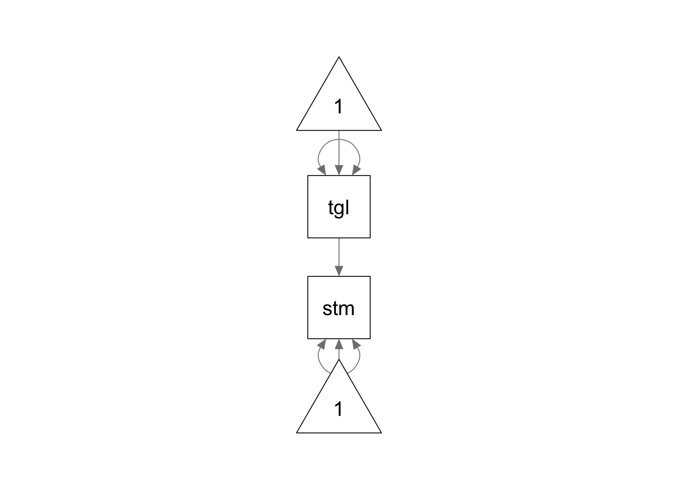
We use the following model syntax to specify the model. The mean structure is specified using ~ 1 command in the model syntax.

model <- '

# direct path
satmath ~ tgoal

# variance 
tgoal ~~ tgoal 
satmath ~~ satmath

# intercept 
tgoal ~ 1
satmath ~ 1

'

fit  <- sem(model, dat)
summary(fit, fit.measures = T, standardized = T)

## lavaan 0.6.15 ended normally after 27 iterations
## 
##   Estimator                                         ML
##   Optimization method                           NLMINB
##   Number of model parameters                         5
## 
##   Number of observations                          1000
## 
## Model Test User Model:
##                                                       
##   Test statistic                                 0.000
##   Degrees of freedom                                 0
## 
## Model Test Baseline Model:
## 
##   Test statistic                                 2.408
##   Degrees of freedom                                 1
##   P-value                                        0.121
## 
## User Model versus Baseline Model:
## 
##   Comparative Fit Index (CFI)                    1.000
##   Tucker-Lewis Index (TLI)                       1.000
## 
## Loglikelihood and Information Criteria:
## 
##   Loglikelihood user model (H0)              -6691.008
##   Loglikelihood unrestricted model (H1)      -6691.008
##                                                       
##   Akaike (AIC)                               13392.016
##   Bayesian (BIC)                             13416.555
##   Sample-size adjusted Bayesian (SABIC)      13400.674
## 
## Root Mean Square Error of Approximation:
## 
##   RMSEA                                          0.000
##   90 Percent confidence interval - lower         0.000
##   90 Percent confidence interval - upper         0.000
##   P-value H_0: RMSEA <= 0.050                       NA
##   P-value H_0: RMSEA >= 0.080                       NA
## 
## Standardized Root Mean Square Residual:
## 
##   SRMR                                           0.000
## 
## Parameter Estimates:
## 
##   Standard errors                             Standard
##   Information                                 Expected
##   Information saturated (h1) model          Structured
## 
## Regressions:
##                    Estimate  Std.Err  z-value  P(>|z|)   Std.lv  Std.all
##   satmath ~                                                             
##     tgoal            -1.428    0.920   -1.553    0.120   -1.428   -0.049
## 
## Intercepts:
##                    Estimate  Std.Err  z-value  P(>|z|)   Std.lv  Std.all
##     tgoal             3.308    0.040   82.159    0.000    3.308    2.598
##    .satmath         690.063    3.259  211.715    0.000  690.063   18.616
## 
## Variances:
##                    Estimate  Std.Err  z-value  P(>|z|)   Std.lv  Std.all
##     tgoal             1.621    0.072   22.361    0.000    1.621    1.000
##    .satmath        1370.779   61.303   22.361    0.000 1370.779    0.998