Nonlinear Latent Growth Models
In this tutorial, we are going to use lavaan to fit
nonlinear latent growth models.
Load the pacakges
library(lavaan)
library(semPlot)
Example: Air Data
Read the data
lower <- '
93.650
79.637 93.564
72.890 87.718 95.732
62.623 76.941 81.886 86.054
53.342 63.803 69.612 70.611 73.666
43.820 50.644 54.443 56.446 58.353 59.154
35.183 41.099 46.016 45.494 49.900 46.163 54.169
39.839 44.099 46.105 44.074 48.345 45.847 49.329 60.528
35.497 39.169 42.262 39.429 42.954 42.950 47.120 54.570 66.183
'

smeans <- c(20.121, 25.521, 29.321, 32.400, 34.186, 35.600, 37.729, 39.029, 38.786)
covmat <- getCov(lower)
rownames(covmat) <- colnames(covmat) <- paste0('V', 1:9)
Linear Model
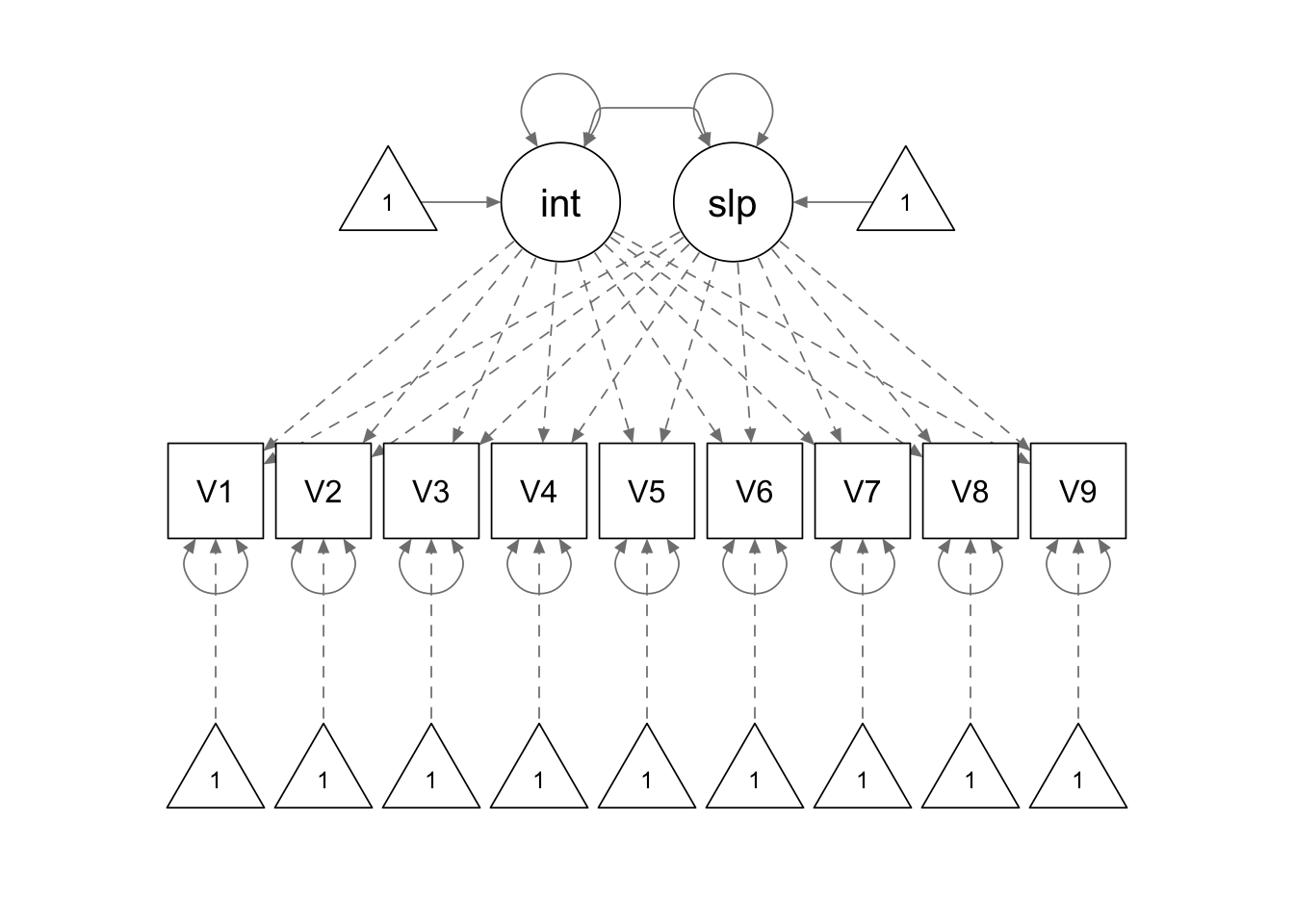
linear.model <- '

interc =~ 1*V1 + 1*V2 + 1*V3 + 1*V4 + 1*V5 + 1*V6 + 1*V7 + 1*V8 + 1*V9
slope =~ 0*V1 + 1*V2 + 2*V3 + 3*V4 + 4*V5 + 5*V6 + 6*V7 + 7*V8 + 8*V9

'

linear.fit <- growth(linear.model, sample.cov=covmat, sample.mean=smeans, sample.nobs = 140)

summary(linear.fit, fit.measures = T)
## lavaan 0.6.15 ended normally after 91 iterations
##
## Estimator ML
## Optimization method NLMINB
## Number of model parameters 14
##
## Number of observations 140
##
## Model Test User Model:
##
## Test statistic 413.528
## Degrees of freedom 40
## P-value (Chi-square) 0.000
##
## Model Test Baseline Model:
##
## Test statistic 1702.962
## Degrees of freedom 36
## P-value 0.000
##
## User Model versus Baseline Model:
##
## Comparative Fit Index (CFI) 0.776
## Tucker-Lewis Index (TLI) 0.798
##
## Loglikelihood and Information Criteria:
##
## Loglikelihood user model (H0) -3851.973
## Loglikelihood unrestricted model (H1) -3645.210
##
## Akaike (AIC) 7731.947
## Bayesian (BIC) 7773.130
## Sample-size adjusted Bayesian (SABIC) 7728.836
##
## Root Mean Square Error of Approximation:
##
## RMSEA 0.258
## 90 Percent confidence interval - lower 0.236
## 90 Percent confidence interval - upper 0.281
## P-value H_0: RMSEA <= 0.050 0.000
## P-value H_0: RMSEA >= 0.080 1.000
##
## Standardized Root Mean Square Residual:
##
## SRMR 0.165
##
## Parameter Estimates:
##
## Standard errors Standard
## Information Expected
## Information saturated (h1) model Structured
##
## Latent Variables:
## Estimate Std.Err z-value P(>|z|)
## interc =~
## V1 1.000
## V2 1.000
## V3 1.000
## V4 1.000
## V5 1.000
## V6 1.000
## V7 1.000
## V8 1.000
## V9 1.000
## slope =~
## V1 0.000
## V2 1.000
## V3 2.000
## V4 3.000
## V5 4.000
## V6 5.000
## V7 6.000
## V8 7.000
## V9 8.000
##
## Covariances:
## Estimate Std.Err z-value P(>|z|)
## interc ~~
## slope -9.629 1.526 -6.311 0.000
##
## Intercepts:
## Estimate Std.Err z-value P(>|z|)
## .V1 0.000
## .V2 0.000
## .V3 0.000
## .V4 0.000
## .V5 0.000
## .V6 0.000
## .V7 0.000
## .V8 0.000
## .V9 0.000
## interc 24.599 0.902 27.279 0.000
## slope 2.114 0.115 18.443 0.000
##
## Variances:
## Estimate Std.Err z-value P(>|z|)
## .V1 59.014 7.787 7.579 0.000
## .V2 11.063 2.057 5.378 0.000
## .V3 8.568 1.486 5.764 0.000
## .V4 14.757 2.002 7.372 0.000
## .V5 12.952 1.733 7.473 0.000
## .V6 12.023 1.639 7.334 0.000
## .V7 8.774 1.375 6.379 0.000
## .V8 8.675 1.612 5.381 0.000
## .V9 25.644 3.728 6.878 0.000
## interc 107.692 13.615 7.910 0.000
## slope 1.574 0.220 7.139 0.000Quadratic Model
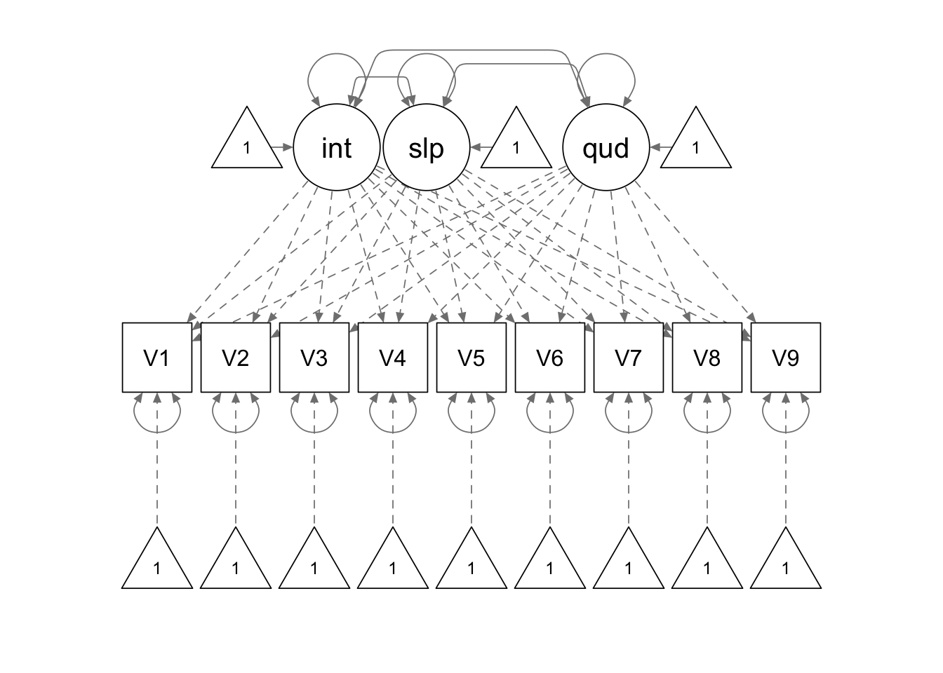
quad.model <- '

interc =~ 1*V1 + 1*V2 + 1*V3 + 1*V4 + 1*V5 + 1*V6 + 1*V7 + 1*V8 + 1*V9
slope =~ 0*V1 + 1*V2 + 2*V3 + 3*V4 + 4*V5 + 5*V6 + 6*V7 + 7*V8 + 8*V9
quad =~ 0*V1 + 1*V2 + 4*V3 + 9*V4 + 16*V5 + 25*V6 + 36*V7 + 49*V8 + 64*V9

'

quad.fit <- growth(quad.model, sample.cov=covmat, sample.mean=smeans, sample.nobs = 140)

summary(quad.fit, fit.measures = T)
## lavaan 0.6.15 ended normally after 108 iterations
##
## Estimator ML
## Optimization method NLMINB
## Number of model parameters 18
##
## Number of observations 140
##
## Model Test User Model:
##
## Test statistic 154.710
## Degrees of freedom 36
## P-value (Chi-square) 0.000
##
## Model Test Baseline Model:
##
## Test statistic 1702.962
## Degrees of freedom 36
## P-value 0.000
##
## User Model versus Baseline Model:
##
## Comparative Fit Index (CFI) 0.929
## Tucker-Lewis Index (TLI) 0.929
##
## Loglikelihood and Information Criteria:
##
## Loglikelihood user model (H0) -3722.565
## Loglikelihood unrestricted model (H1) -3645.210
##
## Akaike (AIC) 7481.129
## Bayesian (BIC) 7534.079
## Sample-size adjusted Bayesian (SABIC) 7477.129
##
## Root Mean Square Error of Approximation:
##
## RMSEA 0.153
## 90 Percent confidence interval - lower 0.129
## 90 Percent confidence interval - upper 0.179
## P-value H_0: RMSEA <= 0.050 0.000
## P-value H_0: RMSEA >= 0.080 1.000
##
## Standardized Root Mean Square Residual:
##
## SRMR 0.104
##
## Parameter Estimates:
##
## Standard errors Standard
## Information Expected
## Information saturated (h1) model Structured
##
## Latent Variables:
## Estimate Std.Err z-value P(>|z|)
## interc =~
## V1 1.000
## V2 1.000
## V3 1.000
## V4 1.000
## V5 1.000
## V6 1.000
## V7 1.000
## V8 1.000
## V9 1.000
## slope =~
## V1 0.000
## V2 1.000
## V3 2.000
## V4 3.000
## V5 4.000
## V6 5.000
## V7 6.000
## V8 7.000
## V9 8.000
## quad =~
## V1 0.000
## V2 1.000
## V3 4.000
## V4 9.000
## V5 16.000
## V6 25.000
## V7 36.000
## V8 49.000
## V9 64.000
##
## Covariances:
## Estimate Std.Err z-value P(>|z|)
## interc ~~
## slope -15.556 3.359 -4.631 0.000
## quad 0.777 0.336 2.315 0.021
## slope ~~
## quad -0.730 0.129 -5.674 0.000
##
## Intercepts:
## Estimate Std.Err z-value P(>|z|)
## .V1 0.000
## .V2 0.000
## .V3 0.000
## .V4 0.000
## .V5 0.000
## .V6 0.000
## .V7 0.000
## .V8 0.000
## .V9 0.000
## interc 21.348 0.918 23.260 0.000
## slope 4.347 0.267 16.257 0.000
## quad -0.269 0.029 -9.188 0.000
##
## Variances:
## Estimate Std.Err z-value P(>|z|)
## .V1 29.757 4.655 6.393 0.000
## .V2 3.418 1.264 2.705 0.007
## .V3 9.360 1.350 6.935 0.000
## .V4 10.315 1.472 7.008 0.000
## .V5 6.778 1.140 5.946 0.000
## .V6 10.089 1.485 6.794 0.000
## .V7 9.474 1.377 6.882 0.000
## .V8 8.254 1.416 5.828 0.000
## .V9 7.344 2.441 3.009 0.003
## interc 111.181 14.160 7.852 0.000
## slope 7.587 1.220 6.221 0.000
## quad 0.088 0.015 5.902 0.000Spline Model-1

spline.model1 <- '

interc =~ 1*V1 + 1*V2 + 1*V3 + 1*V4 + 1*V5 + 1*V6 + 1*V7 + 1*V8 + 1*V9
slope1 =~ 0*V1 + 1*V2 + 2*V3 + 3*V4 + 4*V5 + 4*V6 + 4*V7 + 4*V8 + 4*V9
slope2 =~ 0*V1 + 0*V2 + 0*V3 + 0*V4 + 0*V5 + 1*V6 + 2*V7 + 3*V8 + 4*V9

'

spline.fit1 <- growth(spline.model1, sample.cov = covmat, sample.mean = smeans, sample.nobs = 140)

summary(spline.fit1, fit.measures = T)
## lavaan 0.6.15 ended normally after 117 iterations
##
## Estimator ML
## Optimization method NLMINB
## Number of model parameters 18
##
## Number of observations 140
##
## Model Test User Model:
##
## Test statistic 172.011
## Degrees of freedom 36
## P-value (Chi-square) 0.000
##
## Model Test Baseline Model:
##
## Test statistic 1702.962
## Degrees of freedom 36
## P-value 0.000
##
## User Model versus Baseline Model:
##
## Comparative Fit Index (CFI) 0.918
## Tucker-Lewis Index (TLI) 0.918
##
## Loglikelihood and Information Criteria:
##
## Loglikelihood user model (H0) -3731.215
## Loglikelihood unrestricted model (H1) -3645.210
##
## Akaike (AIC) 7498.430
## Bayesian (BIC) 7551.379
## Sample-size adjusted Bayesian (SABIC) 7494.430
##
## Root Mean Square Error of Approximation:
##
## RMSEA 0.164
## 90 Percent confidence interval - lower 0.140
## 90 Percent confidence interval - upper 0.189
## P-value H_0: RMSEA <= 0.050 0.000
## P-value H_0: RMSEA >= 0.080 1.000
##
## Standardized Root Mean Square Residual:
##
## SRMR 0.119
##
## Parameter Estimates:
##
## Standard errors Standard
## Information Expected
## Information saturated (h1) model Structured
##
## Latent Variables:
## Estimate Std.Err z-value P(>|z|)
## interc =~
## V1 1.000
## V2 1.000
## V3 1.000
## V4 1.000
## V5 1.000
## V6 1.000
## V7 1.000
## V8 1.000
## V9 1.000
## slope1 =~
## V1 0.000
## V2 1.000
## V3 2.000
## V4 3.000
## V5 4.000
## V6 4.000
## V7 4.000
## V8 4.000
## V9 4.000
## slope2 =~
## V1 0.000
## V2 0.000
## V3 0.000
## V4 0.000
## V5 0.000
## V6 1.000
## V7 2.000
## V8 3.000
## V9 4.000
##
## Covariances:
## Estimate Std.Err z-value P(>|z|)
## interc ~~
## slope1 -12.985 2.243 -5.790 0.000
## slope2 -6.891 1.807 -3.813 0.000
## slope1 ~~
## slope2 -0.125 0.335 -0.374 0.708
##
## Intercepts:
## Estimate Std.Err z-value P(>|z|)
## .V1 0.000
## .V2 0.000
## .V3 0.000
## .V4 0.000
## .V5 0.000
## .V6 0.000
## .V7 0.000
## .V8 0.000
## .V9 0.000
## interc 22.458 0.908 24.727 0.000
## slope1 3.048 0.172 17.693 0.000
## slope2 1.269 0.160 7.937 0.000
##
## Variances:
## Estimate Std.Err z-value P(>|z|)
## .V1 36.964 5.047 7.324 0.000
## .V2 1.403 1.241 1.130 0.258
## .V3 10.209 1.400 7.292 0.000
## .V4 11.270 1.520 7.414 0.000
## .V5 3.996 1.192 3.353 0.001
## .V6 9.389 1.337 7.021 0.000
## .V7 9.575 1.353 7.076 0.000
## .V8 7.067 1.384 5.106 0.000
## .V9 11.736 2.438 4.814 0.000
## interc 112.909 13.915 8.114 0.000
## slope1 3.697 0.516 7.160 0.000
## slope2 2.949 0.435 6.782 0.000Spline Model-2
spline.model2 <- '

interc =~ 1*V1 + 1*V2 + 1*V3 + 1*V4 + 1*V5 + 1*V6 + 1*V7 + 1*V8 + 1*V9
slope1 =~ 0*V1 + 1*V2 + 2*V3 + 3*V4 + 3*V5 + 3*V6 + 3*V7 + 3*V8 + 3*V9
slope2 =~ 0*V1 + 0*V2 + 0*V3 + 0*V4 + 1*V5 + 2*V6 + 3*V7 + 4*V8 + 5*V9

'

spline.fit2 <- growth(spline.model2, sample.cov = covmat, sample.mean = smeans, sample.nobs = 140)

summary(spline.fit2, fit.measures = T)
## lavaan 0.6.15 ended normally after 109 iterations
##
## Estimator ML
## Optimization method NLMINB
## Number of model parameters 18
##
## Number of observations 140
##
## Model Test User Model:
##
## Test statistic 158.440
## Degrees of freedom 36
## P-value (Chi-square) 0.000
##
## Model Test Baseline Model:
##
## Test statistic 1702.962
## Degrees of freedom 36
## P-value 0.000
##
## User Model versus Baseline Model:
##
## Comparative Fit Index (CFI) 0.927
## Tucker-Lewis Index (TLI) 0.927
##
## Loglikelihood and Information Criteria:
##
## Loglikelihood user model (H0) -3724.429
## Loglikelihood unrestricted model (H1) -3645.210
##
## Akaike (AIC) 7484.859
## Bayesian (BIC) 7537.809
## Sample-size adjusted Bayesian (SABIC) 7480.859
##
## Root Mean Square Error of Approximation:
##
## RMSEA 0.156
## 90 Percent confidence interval - lower 0.132
## 90 Percent confidence interval - upper 0.181
## P-value H_0: RMSEA <= 0.050 0.000
## P-value H_0: RMSEA >= 0.080 1.000
##
## Standardized Root Mean Square Residual:
##
## SRMR 0.089
##
## Parameter Estimates:
##
## Standard errors Standard
## Information Expected
## Information saturated (h1) model Structured
##
## Latent Variables:
## Estimate Std.Err z-value P(>|z|)
## interc =~
## V1 1.000
## V2 1.000
## V3 1.000
## V4 1.000
## V5 1.000
## V6 1.000
## V7 1.000
## V8 1.000
## V9 1.000
## slope1 =~
## V1 0.000
## V2 1.000
## V3 2.000
## V4 3.000
## V5 3.000
## V6 3.000
## V7 3.000
## V8 3.000
## V9 3.000
## slope2 =~
## V1 0.000
## V2 0.000
## V3 0.000
## V4 0.000
## V5 1.000
## V6 2.000
## V7 3.000
## V8 4.000
## V9 5.000
##
## Covariances:
## Estimate Std.Err z-value P(>|z|)
## interc ~~
## slope1 -9.999 2.432 -4.112 0.000
## slope2 -7.849 1.671 -4.697 0.000
## slope1 ~~
## slope2 -0.363 0.374 -0.970 0.332
##
## Intercepts:
## Estimate Std.Err z-value P(>|z|)
## .V1 0.000
## .V2 0.000
## .V3 0.000
## .V4 0.000
## .V5 0.000
## .V6 0.000
## .V7 0.000
## .V8 0.000
## .V9 0.000
## interc 21.471 0.876 24.508 0.000
## slope1 3.781 0.205 18.429 0.000
## slope2 1.449 0.149 9.695 0.000
##
## Variances:
## Estimate Std.Err z-value P(>|z|)
## .V1 25.455 4.207 6.051 0.000
## .V2 4.277 1.350 3.169 0.002
## .V3 8.643 1.272 6.797 0.000
## .V4 6.259 1.376 4.548 0.000
## .V5 7.983 1.219 6.548 0.000
## .V6 11.116 1.500 7.411 0.000
## .V7 9.711 1.397 6.952 0.000
## .V8 6.363 1.353 4.703 0.000
## .V9 15.523 2.682 5.788 0.000
## interc 100.209 12.905 7.765 0.000
## slope1 4.339 0.725 5.984 0.000
## slope2 2.676 0.376 7.119 0.000Spline Model-3
spline.model3 <- '

interc =~ 1*V1 + 1*V2 + 1*V3 + 1*V4 + 1*V5 + 1*V6 + 1*V7 + 1*V8 + 1*V9
slope1 =~ 0*V1 + 1*V2 + 2*V3 + 2*V4 + 2*V5 + 2*V6 + 2*V7 + 2*V8 + 2*V9
slope2 =~ 0*V1 + 0*V2 + 0*V3 + 1*V4 + 2*V5 + 3*V6 + 4*V7 + 5*V8 + 6*V9

'

spline.fit3 <- growth(spline.model3, sample.cov = covmat, sample.mean = smeans, sample.nobs = 140)

summary(spline.fit3, fit.measures = T)
## lavaan 0.6.15 ended normally after 103 iterations
##
## Estimator ML
## Optimization method NLMINB
## Number of model parameters 18
##
## Number of observations 140
##
## Model Test User Model:
##
## Test statistic 205.005
## Degrees of freedom 36
## P-value (Chi-square) 0.000
##
## Model Test Baseline Model:
##
## Test statistic 1702.962
## Degrees of freedom 36
## P-value 0.000
##
## User Model versus Baseline Model:
##
## Comparative Fit Index (CFI) 0.899
## Tucker-Lewis Index (TLI) 0.899
##
## Loglikelihood and Information Criteria:
##
## Loglikelihood user model (H0) -3747.712
## Loglikelihood unrestricted model (H1) -3645.210
##
## Akaike (AIC) 7531.425
## Bayesian (BIC) 7584.374
## Sample-size adjusted Bayesian (SABIC) 7527.425
##
## Root Mean Square Error of Approximation:
##
## RMSEA 0.183
## 90 Percent confidence interval - lower 0.159
## 90 Percent confidence interval - upper 0.208
## P-value H_0: RMSEA <= 0.050 0.000
## P-value H_0: RMSEA >= 0.080 1.000
##
## Standardized Root Mean Square Residual:
##
## SRMR 0.067
##
## Parameter Estimates:
##
## Standard errors Standard
## Information Expected
## Information saturated (h1) model Structured
##
## Latent Variables:
## Estimate Std.Err z-value P(>|z|)
## interc =~
## V1 1.000
## V2 1.000
## V3 1.000
## V4 1.000
## V5 1.000
## V6 1.000
## V7 1.000
## V8 1.000
## V9 1.000
## slope1 =~
## V1 0.000
## V2 1.000
## V3 2.000
## V4 2.000
## V5 2.000
## V6 2.000
## V7 2.000
## V8 2.000
## V9 2.000
## slope2 =~
## V1 0.000
## V2 0.000
## V3 0.000
## V4 1.000
## V5 2.000
## V6 3.000
## V7 4.000
## V8 5.000
## V9 6.000
##
## Covariances:
## Estimate Std.Err z-value P(>|z|)
## interc ~~
## slope1 -7.769 3.312 -2.346 0.019
## slope2 -6.923 1.424 -4.862 0.000
## slope1 ~~
## slope2 -1.240 0.500 -2.480 0.013
##
## Intercepts:
## Estimate Std.Err z-value P(>|z|)
## .V1 0.000
## .V2 0.000
## .V3 0.000
## .V4 0.000
## .V5 0.000
## .V6 0.000
## .V7 0.000
## .V8 0.000
## .V9 0.000
## interc 20.240 0.819 24.716 0.000
## slope1 5.085 0.295 17.250 0.000
## slope2 1.683 0.135 12.507 0.000
##
## Variances:
## Estimate Std.Err z-value P(>|z|)
## .V1 9.866 3.834 2.573 0.010
## .V2 8.111 1.520 5.337 0.000
## .V3 10.681 1.942 5.498 0.000
## .V4 8.502 1.391 6.111 0.000
## .V5 9.845 1.386 7.105 0.000
## .V6 11.624 1.567 7.417 0.000
## .V7 9.474 1.398 6.776 0.000
## .V8 6.857 1.404 4.884 0.000
## .V9 18.589 2.950 6.301 0.000
## interc 86.088 11.453 7.517 0.000
## slope1 8.661 1.647 5.260 0.000
## slope2 2.174 0.304 7.150 0.000Spline Model-4
spline.model4 <- '

interc =~ 1*V1 + 1*V2 + 1*V3 + 1*V4 + 1*V5 + 1*V6 + 1*V7 + 1*V8 + 1*V9
slope1 =~ 0*V1 + 1*V2 + 2*V3 + 2*V4 + 2*V5 + 2*V6 + 2*V7 + 2*V8 + 2*V9
slope2 =~ 0*V1 + 0*V2 + 0*V3 + 1*V4 + 2*V5 + 3*V6 + 4*V7 + 5*V8 + 6*V9
slope3 =~ 0*V1 + 0*V2 + 0*V3 + 0*V4 + 0*V5 + 0*V6 + 1*V7 + 2*V8 + 3*V9

'

spline.fit4 <- growth(spline.model4, sample.cov = covmat, sample.mean = smeans, sample.nobs = 140)

summary(spline.fit4, fit.measures = T)
## lavaan 0.6.15 ended normally after 144 iterations
##
## Estimator ML
## Optimization method NLMINB
## Number of model parameters 23
##
## Number of observations 140
##
## Model Test User Model:
##
## Test statistic 100.459
## Degrees of freedom 31
## P-value (Chi-square) 0.000
##
## Model Test Baseline Model:
##
## Test statistic 1702.962
## Degrees of freedom 36
## P-value 0.000
##
## User Model versus Baseline Model:
##
## Comparative Fit Index (CFI) 0.958
## Tucker-Lewis Index (TLI) 0.952
##
## Loglikelihood and Information Criteria:
##
## Loglikelihood user model (H0) -3695.439
## Loglikelihood unrestricted model (H1) -3645.210
##
## Akaike (AIC) 7436.878
## Bayesian (BIC) 7504.536
## Sample-size adjusted Bayesian (SABIC) 7431.767
##
## Root Mean Square Error of Approximation:
##
## RMSEA 0.127
## 90 Percent confidence interval - lower 0.099
## 90 Percent confidence interval - upper 0.155
## P-value H_0: RMSEA <= 0.050 0.000
## P-value H_0: RMSEA >= 0.080 0.997
##
## Standardized Root Mean Square Residual:
##
## SRMR 0.045
##
## Parameter Estimates:
##
## Standard errors Standard
## Information Expected
## Information saturated (h1) model Structured
##
## Latent Variables:
## Estimate Std.Err z-value P(>|z|)
## interc =~
## V1 1.000
## V2 1.000
## V3 1.000
## V4 1.000
## V5 1.000
## V6 1.000
## V7 1.000
## V8 1.000
## V9 1.000
## slope1 =~
## V1 0.000
## V2 1.000
## V3 2.000
## V4 2.000
## V5 2.000
## V6 2.000
## V7 2.000
## V8 2.000
## V9 2.000
## slope2 =~
## V1 0.000
## V2 0.000
## V3 0.000
## V4 1.000
## V5 2.000
## V6 3.000
## V7 4.000
## V8 5.000
## V9 6.000
## slope3 =~
## V1 0.000
## V2 0.000
## V3 0.000
## V4 0.000
## V5 0.000
## V6 0.000
## V7 1.000
## V8 2.000
## V9 3.000
##
## Covariances:
## Estimate Std.Err z-value P(>|z|)
## interc ~~
## slope1 -3.053 2.796 -1.092 0.275
## slope2 -11.537 2.090 -5.520 0.000
## slope3 9.383 2.776 3.381 0.001
## slope1 ~~
## slope2 -0.788 0.678 -1.162 0.245
## slope3 -0.627 0.931 -0.674 0.500
## slope2 ~~
## slope3 -3.988 0.822 -4.851 0.000
##
## Intercepts:
## Estimate Std.Err z-value P(>|z|)
## .V1 0.000
## .V2 0.000
## .V3 0.000
## .V4 0.000
## .V5 0.000
## .V6 0.000
## .V7 0.000
## .V8 0.000
## .V9 0.000
## interc 20.653 0.815 25.332 0.000
## slope1 4.497 0.266 16.880 0.000
## slope2 2.199 0.193 11.400 0.000
## slope3 -1.135 0.276 -4.109 0.000
##
## Variances:
## Estimate Std.Err z-value P(>|z|)
## .V1 16.174 3.680 4.396 0.000
## .V2 5.626 1.240 4.538 0.000
## .V3 4.327 1.466 2.951 0.003
## .V4 10.102 1.427 7.079 0.000
## .V5 7.564 1.149 6.584 0.000
## .V6 7.130 1.513 4.712 0.000
## .V7 8.861 1.318 6.723 0.000
## .V8 7.794 1.408 5.537 0.000
## .V9 9.037 2.474 3.653 0.000
## interc 83.075 11.205 7.414 0.000
## slope1 5.939 1.351 4.396 0.000
## slope2 4.256 0.641 6.634 0.000
## slope3 7.016 1.356 5.173 0.000Unspecified Loadings
model5 <- '

interc =~ 1*V1 + 1*V2 + 1*V3 + 1*V4 + 1*V5 + 1*V6 + 1*V7 + 1*V8 + 1*V9
slope =~ 0*V1 + 1*V2 + NA*V3 + NA*V4 + NA*V5 + NA*V6 + NA*V7 + NA*V8 + NA*V9

'

fit5 <- growth(model5, sample.cov = covmat, sample.mean = smeans, sample.nobs = 140)

summary(fit5, fit.measures = T)
## lavaan 0.6.15 ended normally after 96 iterations
##
## Estimator ML
## Optimization method NLMINB
## Number of model parameters 21
##
## Number of observations 140
##
## Model Test User Model:
##
## Test statistic 276.817
## Degrees of freedom 33
## P-value (Chi-square) 0.000
##
## Model Test Baseline Model:
##
## Test statistic 1702.962
## Degrees of freedom 36
## P-value 0.000
##
## User Model versus Baseline Model:
##
## Comparative Fit Index (CFI) 0.854
## Tucker-Lewis Index (TLI) 0.840
##
## Loglikelihood and Information Criteria:
##
## Loglikelihood user model (H0) -3783.618
## Loglikelihood unrestricted model (H1) -3645.210
##
## Akaike (AIC) 7609.236
## Bayesian (BIC) 7671.011
## Sample-size adjusted Bayesian (SABIC) 7604.570
##
## Root Mean Square Error of Approximation:
##
## RMSEA 0.230
## 90 Percent confidence interval - lower 0.205
## 90 Percent confidence interval - upper 0.255
## P-value H_0: RMSEA <= 0.050 0.000
## P-value H_0: RMSEA >= 0.080 1.000
##
## Standardized Root Mean Square Residual:
##
## SRMR 0.134
##
## Parameter Estimates:
##
## Standard errors Standard
## Information Expected
## Information saturated (h1) model Structured
##
## Latent Variables:
## Estimate Std.Err z-value P(>|z|)
## interc =~
## V1 1.000
## V2 1.000
## V3 1.000
## V4 1.000
## V5 1.000
## V6 1.000
## V7 1.000
## V8 1.000
## V9 1.000
## slope =~
## V1 0.000
## V2 1.000
## V3 1.872 0.144 13.018 0.000
## V4 2.635 0.236 11.177 0.000
## V5 3.227 0.304 10.623 0.000
## V6 3.657 0.355 10.287 0.000
## V7 4.245 0.426 9.958 0.000
## V8 4.499 0.459 9.798 0.000
## V9 4.499 0.463 9.721 0.000
##
## Covariances:
## Estimate Std.Err z-value P(>|z|)
## interc ~~
## slope -17.920 3.803 -4.712 0.000
##
## Intercepts:
## Estimate Std.Err z-value P(>|z|)
## .V1 0.000
## .V2 0.000
## .V3 0.000
## .V4 0.000
## .V5 0.000
## .V6 0.000
## .V7 0.000
## .V8 0.000
## .V9 0.000
## interc 21.658 1.042 20.777 0.000
## slope 3.848 0.518 7.423 0.000
##
## Variances:
## Estimate Std.Err z-value P(>|z|)
## .V1 36.932 5.210 7.089 0.000
## .V2 3.583 1.410 2.541 0.011
## .V3 10.788 1.539 7.008 0.000
## .V4 16.544 2.122 7.797 0.000
## .V5 12.823 1.696 7.562 0.000
## .V6 11.437 1.580 7.239 0.000
## .V7 7.488 1.284 5.834 0.000
## .V8 10.658 1.702 6.263 0.000
## .V9 19.512 2.698 7.233 0.000
## interc 121.309 15.592 7.780 0.000
## slope 4.444 1.254 3.544 0.000Example: Antisocial Data
Read the data
setwd(mypath)  # change it to the path of your own data folder

dat <- read.table("Read-Data-Mplus.dat", sep = "\t", header = F, na.strings = "-99")

colnames(dat) <-c('id', 'gen', 'momage', 'homecog', 'homeemo', paste0('an', 1:4), paste0('r', 1:4), paste0('ag', 1:4))

# check the data
str(dat)
## 'data.frame': 405 obs. of 17 variables:
## $ id : int 1 2 3 4 5 6 7 8 9 10 ...
## $ gen : int 1 1 0 1 1 0 0 0 0 0 ...
## $ momage : int 27 27 27 24 26 25 22 23 24 28 ...
## $ homecog: int 7 10 7 8 8 6 5 1 3 9 ...
## $ homeemo: int 11 7 7 8 8 11 5 4 7 11 ...
## $ an1 : int 1 1 5 1 2 1 3 0 5 2 ...
## $ an2 : int 0 1 0 1 3 0 NA NA 3 3 ...
## $ an3 : int 1 0 5 NA 3 0 0 0 2 6 ...
## $ an4 : int 0 1 3 NA 1 0 10 4 0 5 ...
## $ r1 : int 27 31 36 18 23 21 21 13 29 45 ...
## $ r2 : int 49 47 52 30 49 NA NA NA NA 58 ...
## $ r3 : int 50 56 60 NA NA 45 48 37 35 76 ...
## $ r4 : int NA 64 75 NA 77 53 NA NA 38 80 ...
## $ ag1 : int 6 7 8 7 6 6 7 6 8 8 ...
## $ ag2 : int 9 10 11 10 9 9 NA NA 10 10 ...
## $ ag3 : int 11 12 13 NA 11 11 11 10 12 12 ...
## $ ag4 : int 13 14 14 NA 13 13 13 12 14 15 ...summary(dat)## id gen momage homecog
## Min. : 1 Min. :0.0000 Min. :21.00 Min. : 1.000
## 1st Qu.:102 1st Qu.:0.0000 1st Qu.:24.00 1st Qu.: 7.000
## Median :203 Median :1.0000 Median :26.00 Median : 9.000
## Mean :203 Mean :0.5012 Mean :25.53 Mean : 8.894
## 3rd Qu.:304 3rd Qu.:1.0000 3rd Qu.:27.00 3rd Qu.:11.000
## Max. :405 Max. :1.0000 Max. :29.00 Max. :14.000
##
## homeemo an1 an2 an3
## Min. : 0.000 Min. :0.000 Min. : 0.000 Min. : 0.000
## 1st Qu.: 8.000 1st Qu.:0.000 1st Qu.: 0.000 1st Qu.: 0.000
## Median :10.000 Median :1.000 Median : 1.500 Median : 1.000
## Mean : 9.205 Mean :1.662 Mean : 2.027 Mean : 1.828
## 3rd Qu.:11.000 3rd Qu.:3.000 3rd Qu.: 3.000 3rd Qu.: 3.000
## Max. :13.000 Max. :9.000 Max. :10.000 Max. :10.000
## NA's :31 NA's :108
## an4 r1 r2 r3
## Min. : 0.000 Min. : 1.00 Min. :16.00 Min. :22.00
## 1st Qu.: 0.000 1st Qu.:18.00 1st Qu.:33.00 1st Qu.:42.00
## Median : 1.500 Median :23.00 Median :41.00 Median :50.00
## Mean : 2.061 Mean :25.23 Mean :40.76 Mean :50.05
## 3rd Qu.: 3.000 3rd Qu.:30.00 3rd Qu.:49.00 3rd Qu.:58.00
## Max. :10.000 Max. :72.00 Max. :82.00 Max. :84.00
## NA's :111 NA's :30 NA's :130
## r4 ag1 ag2 ag3
## Min. :25.00 Min. :6.000 Min. : 8.000 Min. :10.00
## 1st Qu.:49.25 1st Qu.:6.000 1st Qu.: 9.000 1st Qu.:11.00
## Median :58.00 Median :7.000 Median : 9.000 Median :11.00
## Mean :57.74 Mean :6.983 Mean : 9.353 Mean :11.43
## 3rd Qu.:66.75 3rd Qu.:8.000 3rd Qu.:10.000 3rd Qu.:12.00
## Max. :83.00 Max. :8.000 Max. :11.000 Max. :13.00
## NA's :135 NA's :31 NA's :108
## ag4
## Min. :12.0
## 1st Qu.:13.0
## Median :13.0
## Mean :13.3
## 3rd Qu.:14.0
## Max. :15.0
## NA's :111Linear Model
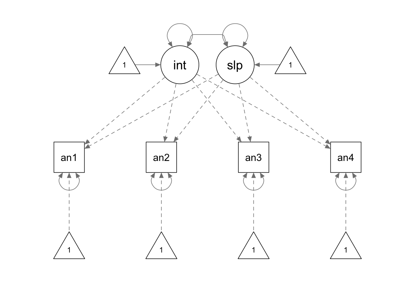
linear.model <- '

interc =~ 1*an1 + 1*an2 + 1*an3 + 1*an4
slope =~ 0*an1 + 1*an2 + 2*an3 + 3*an4

'

linear.fit <- growth(linear.model, dat, missing = "fiml")

summary(linear.fit, fit.measures = T)
## lavaan 0.6.15 ended normally after 32 iterations
##
## Estimator ML
## Optimization method NLMINB
## Number of model parameters 9
##
## Number of observations 405
## Number of missing patterns 8
##
## Model Test User Model:
##
## Test statistic 14.867
## Degrees of freedom 5
## P-value (Chi-square) 0.011
##
## Model Test Baseline Model:
##
## Test statistic 366.752
## Degrees of freedom 6
## P-value 0.000
##
## User Model versus Baseline Model:
##
## Comparative Fit Index (CFI) 0.973
## Tucker-Lewis Index (TLI) 0.967
##
## Robust Comparative Fit Index (CFI) 0.977
## Robust Tucker-Lewis Index (TLI) 0.972
##
## Loglikelihood and Information Criteria:
##
## Loglikelihood user model (H0) -2652.509
## Loglikelihood unrestricted model (H1) -2645.076
##
## Akaike (AIC) 5323.018
## Bayesian (BIC) 5359.053
## Sample-size adjusted Bayesian (SABIC) 5330.495
##
## Root Mean Square Error of Approximation:
##
## RMSEA 0.070
## 90 Percent confidence interval - lower 0.030
## 90 Percent confidence interval - upper 0.112
## P-value H_0: RMSEA <= 0.050 0.177
## P-value H_0: RMSEA >= 0.080 0.387
##
## Robust RMSEA 0.078
## 90 Percent confidence interval - lower 0.029
## 90 Percent confidence interval - upper 0.129
## P-value H_0: Robust RMSEA <= 0.050 0.149
## P-value H_0: Robust RMSEA >= 0.080 0.527
##
## Standardized Root Mean Square Residual:
##
## SRMR 0.053
##
## Parameter Estimates:
##
## Standard errors Standard
## Information Observed
## Observed information based on Hessian
##
## Latent Variables:
## Estimate Std.Err z-value P(>|z|)
## interc =~
## an1 1.000
## an2 1.000
## an3 1.000
## an4 1.000
## slope =~
## an1 0.000
## an2 1.000
## an3 2.000
## an4 3.000
##
## Covariances:
## Estimate Std.Err z-value P(>|z|)
## interc ~~
## slope 0.147 0.092 1.597 0.110
##
## Intercepts:
## Estimate Std.Err z-value P(>|z|)
## .an1 0.000
## .an2 0.000
## .an3 0.000
## .an4 0.000
## interc 1.704 0.079 21.654 0.000
## slope 0.149 0.038 3.912 0.000
##
## Variances:
## Estimate Std.Err z-value P(>|z|)
## .an1 1.587 0.222 7.160 0.000
## .an2 2.064 0.196 10.527 0.000
## .an3 1.533 0.183 8.360 0.000
## .an4 1.604 0.278 5.763 0.000
## interc 1.268 0.215 5.904 0.000
## slope 0.133 0.056 2.384 0.017Quadratic Model
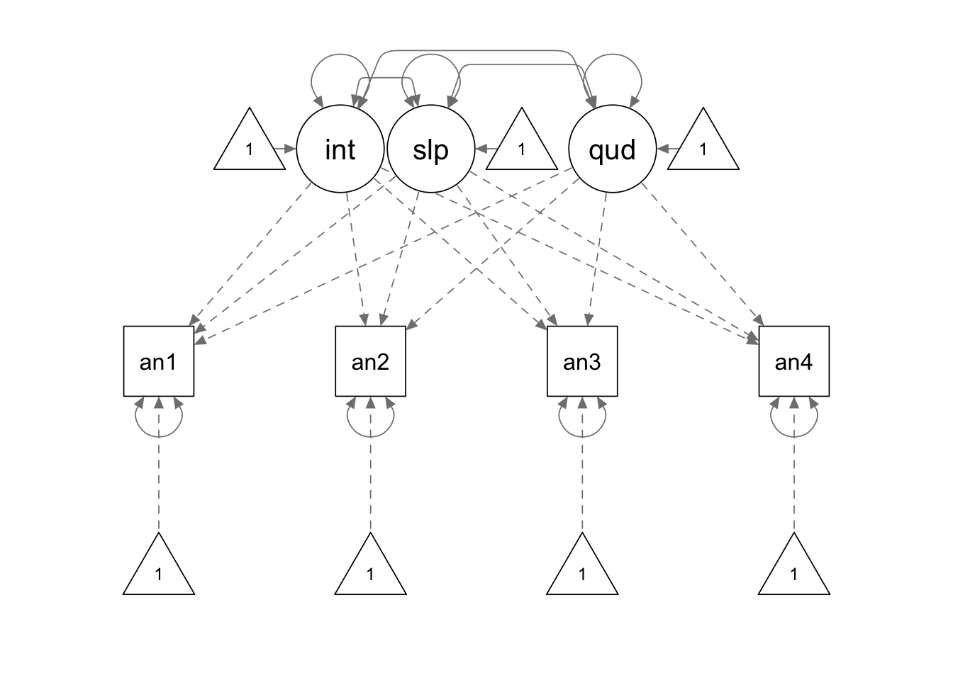
quad.model <- '

interc =~ 1*an1 + 1*an2 + 1*an3 + 1*an4
slope =~ 0*an1 + 1*an2 + 2*an3 + 3*an4
quad =~ 0*an1 + 1*an2 + 4*an3 + 9*an4

'
quad.fit <- growth(quad.model, dat, missing = "fiml")

summary(quad.fit, fit.measures = T)
## lavaan 0.6.15 ended normally after 62 iterations
##
## Estimator ML
## Optimization method NLMINB
## Number of model parameters 13
##
## Number of observations 405
## Number of missing patterns 8
##
## Model Test User Model:
##
## Test statistic 5.405
## Degrees of freedom 1
## P-value (Chi-square) 0.020
##
## Model Test Baseline Model:
##
## Test statistic 366.752
## Degrees of freedom 6
## P-value 0.000
##
## User Model versus Baseline Model:
##
## Comparative Fit Index (CFI) 0.988
## Tucker-Lewis Index (TLI) 0.927
##
## Robust Comparative Fit Index (CFI) 0.989
## Robust Tucker-Lewis Index (TLI) 0.936
##
## Loglikelihood and Information Criteria:
##
## Loglikelihood user model (H0) -2647.778
## Loglikelihood unrestricted model (H1) -2645.076
##
## Akaike (AIC) 5321.557
## Bayesian (BIC) 5373.607
## Sample-size adjusted Bayesian (SABIC) 5332.356
##
## Root Mean Square Error of Approximation:
##
## RMSEA 0.104
## 90 Percent confidence interval - lower 0.033
## 90 Percent confidence interval - upper 0.197
## P-value H_0: RMSEA <= 0.050 0.094
## P-value H_0: RMSEA >= 0.080 0.763
##
## Robust RMSEA 0.117
## 90 Percent confidence interval - lower 0.037
## 90 Percent confidence interval - upper 0.223
## P-value H_0: Robust RMSEA <= 0.050 0.078
## P-value H_0: Robust RMSEA >= 0.080 0.814
##
## Standardized Root Mean Square Residual:
##
## SRMR 0.024
##
## Parameter Estimates:
##
## Standard errors Standard
## Information Observed
## Observed information based on Hessian
##
## Latent Variables:
## Estimate Std.Err z-value P(>|z|)
## interc =~
## an1 1.000
## an2 1.000
## an3 1.000
## an4 1.000
## slope =~
## an1 0.000
## an2 1.000
## an3 2.000
## an4 3.000
## quad =~
## an1 0.000
## an2 1.000
## an3 4.000
## an4 9.000
##
## Covariances:
## Estimate Std.Err z-value P(>|z|)
## interc ~~
## slope -0.478 0.619 -0.773 0.439
## quad 0.125 0.154 0.813 0.416
## slope ~~
## quad -0.012 0.210 -0.055 0.956
##
## Intercepts:
## Estimate Std.Err z-value P(>|z|)
## .an1 0.000
## .an2 0.000
## .an3 0.000
## .an4 0.000
## interc 1.677 0.083 20.320 0.000
## slope 0.202 0.113 1.797 0.072
## quad -0.020 0.036 -0.554 0.580
##
## Variances:
## Estimate Std.Err z-value P(>|z|)
## .an1 0.908 0.552 1.646 0.100
## .an2 2.292 0.273 8.382 0.000
## .an3 1.132 0.234 4.844 0.000
## .an4 3.627 0.839 4.325 0.000
## interc 1.834 0.563 3.261 0.001
## slope 0.799 0.749 1.066 0.286
## quad -0.080 0.075 -1.066 0.286Spline Model-1
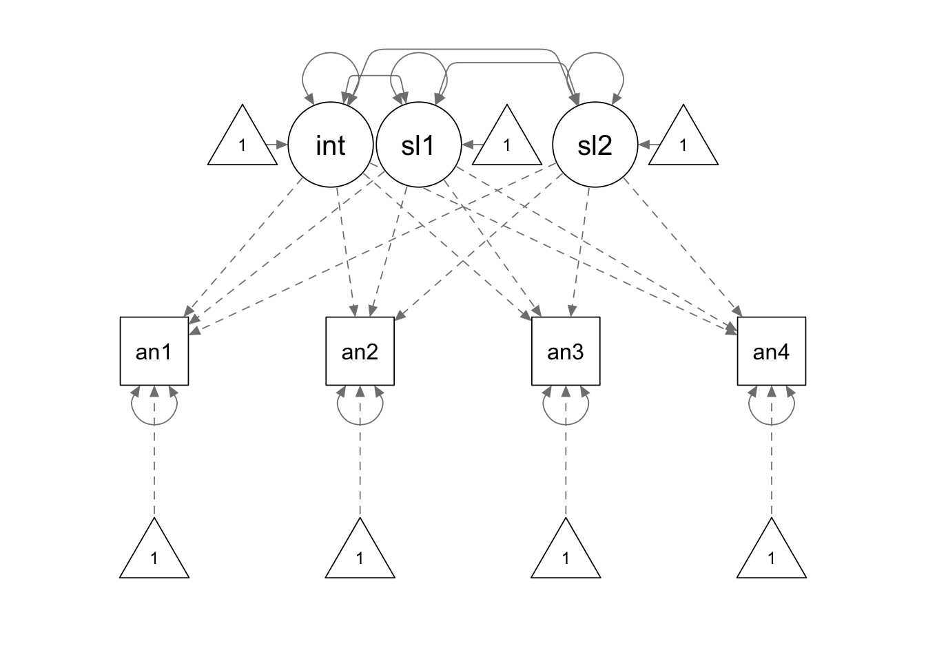
spline.model1 <- '

interc =~ 1*an1 + 1*an2 + 1*an3 + 1*an4
slope1 =~ 0*an1 + 1*an2 + 1*an3 + 1*an4
slope2 =~ 0*an1 + 0*an2 + 1*an3 + 2*an4

an1 ~~ 0*an1
'

spline.fit1 <- growth(spline.model1, dat, missing = "fiml")

summary(spline.fit1, fit.measures = T)
## lavaan 0.6.15 ended normally after 59 iterations
##
## Estimator ML
## Optimization method NLMINB
## Number of model parameters 12
##
## Number of observations 405
## Number of missing patterns 8
##
## Model Test User Model:
##
## Test statistic 4.394
## Degrees of freedom 2
## P-value (Chi-square) 0.111
##
## Model Test Baseline Model:
##
## Test statistic 366.752
## Degrees of freedom 6
## P-value 0.000
##
## User Model versus Baseline Model:
##
## Comparative Fit Index (CFI) 0.993
## Tucker-Lewis Index (TLI) 0.980
##
## Robust Comparative Fit Index (CFI) 0.993
## Robust Tucker-Lewis Index (TLI) 0.980
##
## Loglikelihood and Information Criteria:
##
## Loglikelihood user model (H0) -2647.273
## Loglikelihood unrestricted model (H1) -2645.076
##
## Akaike (AIC) 5318.546
## Bayesian (BIC) 5366.593
## Sample-size adjusted Bayesian (SABIC) 5328.515
##
## Root Mean Square Error of Approximation:
##
## RMSEA 0.054
## 90 Percent confidence interval - lower 0.000
## 90 Percent confidence interval - upper 0.125
## P-value H_0: RMSEA <= 0.050 0.357
## P-value H_0: RMSEA >= 0.080 0.338
##
## Robust RMSEA 0.065
## 90 Percent confidence interval - lower 0.000
## 90 Percent confidence interval - upper 0.148
## P-value H_0: Robust RMSEA <= 0.050 0.283
## P-value H_0: Robust RMSEA >= 0.080 0.469
##
## Standardized Root Mean Square Residual:
##
## SRMR 0.024
##
## Parameter Estimates:
##
## Standard errors Standard
## Information Observed
## Observed information based on Hessian
##
## Latent Variables:
## Estimate Std.Err z-value P(>|z|)
## interc =~
## an1 1.000
## an2 1.000
## an3 1.000
## an4 1.000
## slope1 =~
## an1 0.000
## an2 1.000
## an3 1.000
## an4 1.000
## slope2 =~
## an1 0.000
## an2 0.000
## an3 1.000
## an4 2.000
##
## Covariances:
## Estimate Std.Err z-value P(>|z|)
## interc ~~
## slope1 -1.303 0.170 -7.647 0.000
## slope2 0.018 0.091 0.201 0.841
## slope1 ~~
## slope2 0.369 0.239 1.545 0.122
##
## Intercepts:
## Estimate Std.Err z-value P(>|z|)
## .an1 0.000
## .an2 0.000
## .an3 0.000
## .an4 0.000
## interc 1.662 0.082 20.194 0.000
## slope1 0.268 0.096 2.775 0.006
## slope2 0.086 0.055 1.554 0.120
##
## Variances:
## Estimate Std.Err z-value P(>|z|)
## .an1 0.000
## .an2 2.181 0.404 5.401 0.000
## .an3 1.422 0.186 7.655 0.000
## .an4 2.208 0.417 5.300 0.000
## interc 2.742 0.193 14.230 0.000
## slope1 1.737 0.396 4.384 0.000
## slope2 -0.191 0.208 -0.921 0.357Spline Model-2
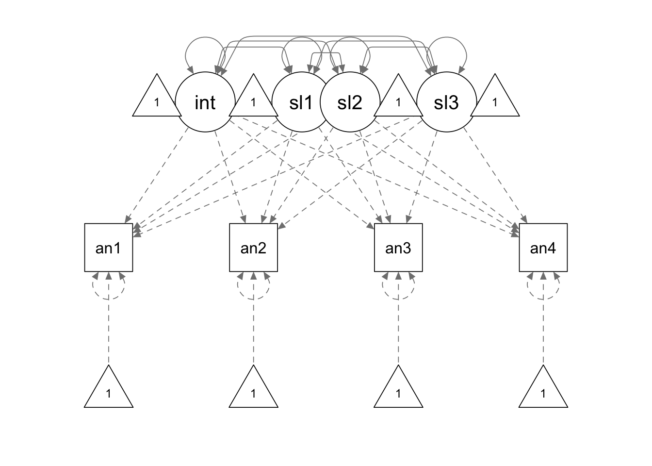
spline.model2 <- '

interc =~ 1*an1 + 1*an2 + 1*an3 + 1*an4
slope1 =~ 0*an1 + 1*an2 + 1*an3 + 1*an4
slope2 =~ 0*an1 + 0*an2 + 1*an3 + 1*an4
slope3 =~ 0*an1 + 0*an2 + 0*an3 + 1*an4

an1 ~~ 0*an1
an2 ~~ 0*an2
an3 ~~ 0*an3
an4 ~~ 0*an4

'

spline.fit2 <- growth(spline.model2, dat, missing = "fiml")


summary(spline.fit2, fit.measures = T)
## lavaan 0.6.15 ended normally after 91 iterations
##
## Estimator ML
## Optimization method NLMINB
## Number of model parameters 14
##
## Number of observations 405
## Number of missing patterns 8
##
## Model Test User Model:
##
## Test statistic 0.000
## Degrees of freedom 0
##
## Model Test Baseline Model:
##
## Test statistic 366.752
## Degrees of freedom 6
## P-value 0.000
##
## User Model versus Baseline Model:
##
## Comparative Fit Index (CFI) 1.000
## Tucker-Lewis Index (TLI) 1.000
##
## Robust Comparative Fit Index (CFI) 1.000
## Robust Tucker-Lewis Index (TLI) 1.000
##
## Loglikelihood and Information Criteria:
##
## Loglikelihood user model (H0) -2645.076
## Loglikelihood unrestricted model (H1) -2645.076
##
## Akaike (AIC) 5318.152
## Bayesian (BIC) 5374.206
## Sample-size adjusted Bayesian (SABIC) 5329.782
##
## Root Mean Square Error of Approximation:
##
## RMSEA 0.000
## 90 Percent confidence interval - lower 0.000
## 90 Percent confidence interval - upper 0.000
## P-value H_0: RMSEA <= 0.050 NA
## P-value H_0: RMSEA >= 0.080 NA
##
## Robust RMSEA 0.000
## 90 Percent confidence interval - lower 0.000
## 90 Percent confidence interval - upper 0.000
## P-value H_0: Robust RMSEA <= 0.050 NA
## P-value H_0: Robust RMSEA >= 0.080 NA
##
## Standardized Root Mean Square Residual:
##
## SRMR 0.000
##
## Parameter Estimates:
##
## Standard errors Standard
## Information Observed
## Observed information based on Hessian
##
## Latent Variables:
## Estimate Std.Err z-value P(>|z|)
## interc =~
## an1 1.000
## an2 1.000
## an3 1.000
## an4 1.000
## slope1 =~
## an1 0.000
## an2 1.000
## an3 1.000
## an4 1.000
## slope2 =~
## an1 0.000
## an2 0.000
## an3 1.000
## an4 1.000
## slope3 =~
## an1 0.000
## an2 0.000
## an3 0.000
## an4 1.000
##
## Covariances:
## Estimate Std.Err z-value P(>|z|)
## interc ~~
## slope1 -1.263 0.176 -7.169 0.000
## slope2 -0.109 0.173 -0.628 0.530
## slope3 0.161 0.182 0.884 0.377
## slope1 ~~
## slope2 -1.766 0.240 -7.364 0.000
## slope3 0.323 0.245 1.320 0.187
## slope2 ~~
## slope3 -1.607 0.244 -6.590 0.000
##
## Intercepts:
## Estimate Std.Err z-value P(>|z|)
## .an1 0.000
## .an2 0.000
## .an3 0.000
## .an4 0.000
## interc 1.662 0.082 20.194 0.000
## slope1 0.328 0.101 3.261 0.001
## slope2 -0.085 0.105 -0.808 0.419
## slope3 0.268 0.109 2.460 0.014
##
## Variances:
## Estimate Std.Err z-value P(>|z|)
## .an1 0.000
## .an2 0.000
## .an3 0.000
## .an4 0.000
## interc 2.742 0.193 14.230 0.000
## slope1 3.873 0.281 13.780 0.000
## slope2 3.411 0.302 11.291 0.000
## slope3 3.420 0.292 11.724 0.000Nonlinear with Specified Loadings
nl.model1 <- '

interc =~ 1*an1 + 1*an2 + 1*an3 + 1*an4
slope =~ 0*an1 + 1*an2 + 1.5*an3 + 1.75*an4

'

nl.fit1 <- growth(nl.model1, dat, missing = "fiml")


summary(nl.fit1, fit.measures = T)
## lavaan 0.6.15 ended normally after 35 iterations
##
## Estimator ML
## Optimization method NLMINB
## Number of model parameters 9
##
## Number of observations 405
## Number of missing patterns 8
##
## Model Test User Model:
##
## Test statistic 9.268
## Degrees of freedom 5
## P-value (Chi-square) 0.099
##
## Model Test Baseline Model:
##
## Test statistic 366.752
## Degrees of freedom 6
## P-value 0.000
##
## User Model versus Baseline Model:
##
## Comparative Fit Index (CFI) 0.988
## Tucker-Lewis Index (TLI) 0.986
##
## Robust Comparative Fit Index (CFI) 0.987
## Robust Tucker-Lewis Index (TLI) 0.985
##
## Loglikelihood and Information Criteria:
##
## Loglikelihood user model (H0) -2649.710
## Loglikelihood unrestricted model (H1) -2645.076
##
## Akaike (AIC) 5317.420
## Bayesian (BIC) 5353.455
## Sample-size adjusted Bayesian (SABIC) 5324.897
##
## Root Mean Square Error of Approximation:
##
## RMSEA 0.046
## 90 Percent confidence interval - lower 0.000
## 90 Percent confidence interval - upper 0.092
## P-value H_0: RMSEA <= 0.050 0.492
## P-value H_0: RMSEA >= 0.080 0.121
##
## Robust RMSEA 0.058
## 90 Percent confidence interval - lower 0.000
## 90 Percent confidence interval - upper 0.113
## P-value H_0: Robust RMSEA <= 0.050 0.344
## P-value H_0: Robust RMSEA >= 0.080 0.293
##
## Standardized Root Mean Square Residual:
##
## SRMR 0.042
##
## Parameter Estimates:
##
## Standard errors Standard
## Information Observed
## Observed information based on Hessian
##
## Latent Variables:
## Estimate Std.Err z-value P(>|z|)
## interc =~
## an1 1.000
## an2 1.000
## an3 1.000
## an4 1.000
## slope =~
## an1 0.000
## an2 1.000
## an3 1.500
## an4 1.750
##
## Covariances:
## Estimate Std.Err z-value P(>|z|)
## interc ~~
## slope 0.159 0.225 0.703 0.482
##
## Intercepts:
## Estimate Std.Err z-value P(>|z|)
## .an1 0.000
## .an2 0.000
## .an3 0.000
## .an4 0.000
## interc 1.673 0.081 20.668 0.000
## slope 0.241 0.061 3.922 0.000
##
## Variances:
## Estimate Std.Err z-value P(>|z|)
## .an1 1.504 0.330 4.564 0.000
## .an2 1.925 0.193 9.972 0.000
## .an3 1.437 0.183 7.859 0.000
## .an4 1.857 0.237 7.840 0.000
## interc 1.269 0.329 3.855 0.000
## slope 0.378 0.175 2.161 0.031Nonlinear with Unspecified Loadings
nl.model2 <- '

interc =~ 1*an1 + 1*an2 + 1*an3 + 1*an4
slope =~ 0*an1 + 1*an2 + an3 + an4

'

nl.fit2 <- growth(nl.model2, dat, missing = "fiml")


summary(nl.fit2, fit.measures = T)
## lavaan 0.6.15 ended normally after 46 iterations
##
## Estimator ML
## Optimization method NLMINB
## Number of model parameters 11
##
## Number of observations 405
## Number of missing patterns 8
##
## Model Test User Model:
##
## Test statistic 0.859
## Degrees of freedom 3
## P-value (Chi-square) 0.835
##
## Model Test Baseline Model:
##
## Test statistic 366.752
## Degrees of freedom 6
## P-value 0.000
##
## User Model versus Baseline Model:
##
## Comparative Fit Index (CFI) 1.000
## Tucker-Lewis Index (TLI) 1.012
##
## Robust Comparative Fit Index (CFI) 1.000
## Robust Tucker-Lewis Index (TLI) 1.011
##
## Loglikelihood and Information Criteria:
##
## Loglikelihood user model (H0) -2645.505
## Loglikelihood unrestricted model (H1) -2645.076
##
## Akaike (AIC) 5313.010
## Bayesian (BIC) 5357.053
## Sample-size adjusted Bayesian (SABIC) 5322.149
##
## Root Mean Square Error of Approximation:
##
## RMSEA 0.000
## 90 Percent confidence interval - lower 0.000
## 90 Percent confidence interval - upper 0.048
## P-value H_0: RMSEA <= 0.050 0.954
## P-value H_0: RMSEA >= 0.080 0.006
##
## Robust RMSEA 0.000
## 90 Percent confidence interval - lower 0.000
## 90 Percent confidence interval - upper 0.057
## P-value H_0: Robust RMSEA <= 0.050 0.933
## P-value H_0: Robust RMSEA >= 0.080 0.016
##
## Standardized Root Mean Square Residual:
##
## SRMR 0.009
##
## Parameter Estimates:
##
## Standard errors Standard
## Information Observed
## Observed information based on Hessian
##
## Latent Variables:
## Estimate Std.Err z-value P(>|z|)
## interc =~
## an1 1.000
## an2 1.000
## an3 1.000
## an4 1.000
## slope =~
## an1 0.000
## an2 1.000
## an3 0.892 0.174 5.115 0.000
## an4 1.574 0.294 5.357 0.000
##
## Covariances:
## Estimate Std.Err z-value P(>|z|)
## interc ~~
## slope 0.218 0.257 0.847 0.397
##
## Intercepts:
## Estimate Std.Err z-value P(>|z|)
## .an1 0.000
## .an2 0.000
## .an3 0.000
## .an4 0.000
## interc 1.654 0.081 20.491 0.000
## slope 0.325 0.086 3.768 0.000
##
## Variances:
## Estimate Std.Err z-value P(>|z|)
## .an1 1.527 0.308 4.955 0.000
## .an2 1.799 0.210 8.556 0.000
## .an3 1.643 0.187 8.769 0.000
## .an4 1.552 0.366 4.240 0.000
## interc 1.224 0.308 3.974 0.000
## slope 0.612 0.266 2.298 0.022© Copyright 2024 @Yi Feng and @Gregory R. Hancock.