More Latent Growth Models
In this tutorial, we are going to use lavaan and
OpenMx to fit more complicated latent growth models.
Load the pacakges
library(lavaan)
library(semPlot)
library(OpenMx)
library(tidyverse)
Example: Model for Aperture (1)
The data for the first example are from 1000 school girls, whose math self-concept has been measured repeatedly at 9th, 10th, 11th, and 12th grade.
Read the data
lower <- '
2.041
1.392  1.901
1.366  1.352  1.665
1.249  1.303  1.348  1.599
'

smeans <- c(3.297, 3.614, 4.042, 4.375)
covmat <- getCov(lower)
rownames(covmat) <- colnames(covmat) <- paste0('mathsc', 9:12)
Fit the model to the data
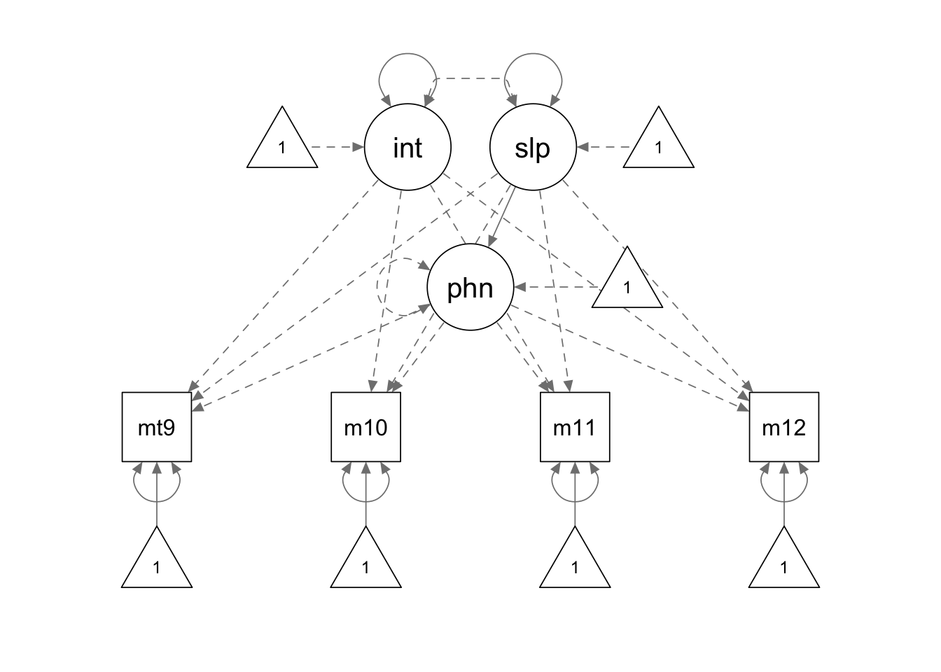
apt.model1 <- '
interc =~ 1*mathsc9 + 1*mathsc10 + 1*mathsc11 + 1*mathsc12
slope =~ 0*mathsc9 + 1*mathsc10 + 2*mathsc11 + 3*mathsc12

# phantom variable
phantom =~ -1*mathsc9 + -1*mathsc10 + -1*mathsc11 + -1*mathsc12
phantom ~~ 0*phantom
phantom ~ slope
interc ~~ 0*slope
'

apt.fit1 <- sem(apt.model1, sample.cov = covmat, sample.mean = smeans, sample.nobs = 1000)
summary(apt.fit1, fit.measures = T, standardized = T)
## lavaan 0.6.15 ended normally after 33 iterations
##
## Estimator ML
## Optimization method NLMINB
## Number of model parameters 11
##
## Number of observations 1000
##
## Model Test User Model:
##
## Test statistic 3.037
## Degrees of freedom 3
## P-value (Chi-square) 0.386
##
## Model Test Baseline Model:
##
## Test statistic 3045.699
## Degrees of freedom 6
## P-value 0.000
##
## User Model versus Baseline Model:
##
## Comparative Fit Index (CFI) 1.000
## Tucker-Lewis Index (TLI) 1.000
##
## Loglikelihood and Information Criteria:
##
## Loglikelihood user model (H0) -5319.933
## Loglikelihood unrestricted model (H1) -5318.415
##
## Akaike (AIC) 10661.867
## Bayesian (BIC) 10715.852
## Sample-size adjusted Bayesian (SABIC) 10680.916
##
## Root Mean Square Error of Approximation:
##
## RMSEA 0.003
## 90 Percent confidence interval - lower 0.000
## 90 Percent confidence interval - upper 0.054
## P-value H_0: RMSEA <= 0.050 0.929
## P-value H_0: RMSEA >= 0.080 0.001
##
## Standardized Root Mean Square Residual:
##
## SRMR 0.008
##
## Parameter Estimates:
##
## Standard errors Standard
## Information Expected
## Information saturated (h1) model Structured
##
## Latent Variables:
## Estimate Std.Err z-value P(>|z|) Std.lv Std.all
## interc =~
## mathsc9 1.000 1.158 0.809
## mathsc10 1.000 1.158 0.838
## mathsc11 1.000 1.158 0.906
## mathsc12 1.000 1.158 0.913
## slope =~
## mathsc9 0.000 0.000 0.000
## mathsc10 1.000 0.190 0.137
## mathsc11 2.000 0.379 0.297
## mathsc12 3.000 0.569 0.448
## phantom =~
## mathsc9 -1.000 -0.379 -0.265
## mathsc10 -1.000 -0.379 -0.274
## mathsc11 -1.000 -0.379 -0.297
## mathsc12 -1.000 -0.379 -0.299
##
## Regressions:
## Estimate Std.Err z-value P(>|z|) Std.lv Std.all
## phantom ~
## slope 1.999 0.368 5.436 0.000 1.000 1.000
##
## Covariances:
## Estimate Std.Err z-value P(>|z|) Std.lv Std.all
## interc ~~
## slope 0.000 0.000 0.000
##
## Intercepts:
## Estimate Std.Err z-value P(>|z|) Std.lv Std.all
## .mathsc9 3.297 0.045 72.813 0.000 3.297 2.303
## .mathsc10 3.614 0.044 82.673 0.000 3.614 2.614
## .mathsc11 4.042 0.040 99.986 0.000 4.042 3.162
## .mathsc12 4.375 0.040 109.011 0.000 4.375 3.447
## interc 0.000 0.000 0.000
## slope 0.000 0.000 0.000
## .phantom 0.000 0.000 0.000
##
## Variances:
## Estimate Std.Err z-value P(>|z|) Std.lv Std.all
## .phantom 0.000 0.000 0.000
## .mathsc9 0.565 0.044 12.795 0.000 0.565 0.275
## .mathsc10 0.533 0.030 17.879 0.000 0.533 0.279
## .mathsc11 0.292 0.020 14.751 0.000 0.292 0.179
## .mathsc12 0.233 0.027 8.546 0.000 0.233 0.145
## interc 1.342 0.064 20.919 0.000 1.000 1.000
## slope 0.036 0.007 4.965 0.000 1.000 1.000Example: Model for Aperture (2)
Read the data
lower <- '
1.000
0.725 1.000
0.595 0.705 1.000
0.566 0.624 0.706 1.000
'

smeans <- c(1.338, 1.591, 2.019, 2.364)
sds <- c(1.260, 1.334, 1.440, 1.376)
covmat <- diag(sds) %*% getCov(lower) %*% diag(sds)
rownames(covmat) <- colnames(covmat) <- paste0('alc', c(12, 14, 16, 18))
Fit the model to the data
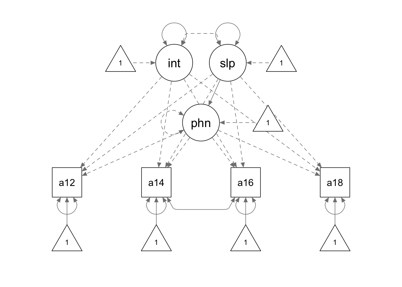
apt.model2 <- '
interc =~ 1*alc12 + 1*alc14 + 1*alc16 + 1*alc18
slope =~ 0*alc12 + 1*alc14 + 2*alc16 + 3*alc18

alc14 ~~ alc16

# phantom variable
phantom =~ -1*alc12 + -1*alc14 + -1*alc16 + -1*alc18
phantom ~~ 0*phantom
phantom ~ slope

# constraints
interc ~~ 0*slope

'
apt.fit2 <- sem(apt.model2, sample.cov = covmat, sample.mean = smeans, sample.nobs = 357)
summary(apt.fit2, fit.measures = T, standardized = F)
## lavaan 0.6.15 ended normally after 29 iterations
##
## Estimator ML
## Optimization method NLMINB
## Number of model parameters 12
##
## Number of observations 357
##
## Model Test User Model:
##
## Test statistic 0.963
## Degrees of freedom 2
## P-value (Chi-square) 0.618
##
## Model Test Baseline Model:
##
## Test statistic 799.900
## Degrees of freedom 6
## P-value 0.000
##
## User Model versus Baseline Model:
##
## Comparative Fit Index (CFI) 1.000
## Tucker-Lewis Index (TLI) 1.004
##
## Loglikelihood and Information Criteria:
##
## Loglikelihood user model (H0) -2054.286
## Loglikelihood unrestricted model (H1) -2053.804
##
## Akaike (AIC) 4132.571
## Bayesian (BIC) 4179.104
## Sample-size adjusted Bayesian (SABIC) 4141.035
##
## Root Mean Square Error of Approximation:
##
## RMSEA 0.000
## 90 Percent confidence interval - lower 0.000
## 90 Percent confidence interval - upper 0.085
## P-value H_0: RMSEA <= 0.050 0.810
## P-value H_0: RMSEA >= 0.080 0.062
##
## Standardized Root Mean Square Residual:
##
## SRMR 0.012
##
## Parameter Estimates:
##
## Standard errors Standard
## Information Expected
## Information saturated (h1) model Structured
##
## Latent Variables:
## Estimate Std.Err z-value P(>|z|)
## interc =~
## alc12 1.000
## alc14 1.000
## alc16 1.000
## alc18 1.000
## slope =~
## alc12 0.000
## alc14 1.000
## alc16 2.000
## alc18 3.000
## phantom =~
## alc12 -1.000
## alc14 -1.000
## alc16 -1.000
## alc18 -1.000
##
## Regressions:
## Estimate Std.Err z-value P(>|z|)
## phantom ~
## slope 1.140 0.237 4.807 0.000
##
## Covariances:
## Estimate Std.Err z-value P(>|z|)
## .alc14 ~~
## .alc16 0.201 0.053 3.769 0.000
## interc ~~
## slope 0.000
##
## Intercepts:
## Estimate Std.Err z-value P(>|z|)
## .alc12 1.338 0.066 20.153 0.000
## .alc14 1.591 0.071 22.269 0.000
## .alc16 2.019 0.077 26.390 0.000
## .alc18 2.364 0.073 32.576 0.000
## interc 0.000
## slope 0.000
## .phantom 0.000
##
## Variances:
## Estimate Std.Err z-value P(>|z|)
## .phantom 0.000
## .alc12 0.214 0.076 2.831 0.005
## .alc14 0.612 0.062 9.886 0.000
## .alc16 0.795 0.076 10.423 0.000
## .alc18 0.270 0.092 2.942 0.003
## interc 1.209 0.100 12.076 0.000
## slope 0.116 0.019 6.235 0.000Example: Definition Variable
In this example, we are going to use OpenMx to employ
definition variables for individually-varying measurement points.
Read the data
setwd(mypath)  # change it to the path of your own data folder

dat <- read.table("growth_antisocial_data.csv", sep = ",", header = F, na.strings = "-99")

colnames(dat) <-c('anti86', 'anti88', 'anti90', 'anti92', 'age86', 'age88', 'age90', 'age92')

# check the data
str(dat)
## 'data.frame': 405 obs. of 8 variables:
## $ anti86: int 1 1 5 1 2 1 3 0 5 2 ...
## $ anti88: int 0 1 0 1 3 0 NA NA 3 3 ...
## $ anti90: int 1 0 5 NA 3 0 0 0 2 6 ...
## $ anti92: int 0 1 3 NA 1 0 10 4 0 5 ...
## $ age86 : int 6 7 8 7 6 6 7 6 8 8 ...
## $ age88 : int 9 10 11 10 9 9 NA NA 10 10 ...
## $ age90 : int 11 12 13 NA 11 11 11 10 12 12 ...
## $ age92 : int 13 14 14 NA 13 13 13 12 14 15 ...summary(dat)## anti86 anti88 anti90 anti92
## Min. :0.000 Min. : 0.000 Min. : 0.000 Min. : 0.000
## 1st Qu.:0.000 1st Qu.: 0.000 1st Qu.: 0.000 1st Qu.: 0.000
## Median :1.000 Median : 1.500 Median : 1.000 Median : 1.500
## Mean :1.662 Mean : 2.027 Mean : 1.828 Mean : 2.061
## 3rd Qu.:3.000 3rd Qu.: 3.000 3rd Qu.: 3.000 3rd Qu.: 3.000
## Max. :9.000 Max. :10.000 Max. :10.000 Max. :10.000
## NA's :31 NA's :108 NA's :111
## age86 age88 age90 age92
## Min. :6.000 Min. : 8.000 Min. :10.00 Min. :12.0
## 1st Qu.:6.000 1st Qu.: 9.000 1st Qu.:11.00 1st Qu.:13.0
## Median :7.000 Median : 9.000 Median :11.00 Median :13.0
## Mean :6.983 Mean : 9.353 Mean :11.43 Mean :13.3
## 3rd Qu.:8.000 3rd Qu.:10.000 3rd Qu.:12.00 3rd Qu.:14.0
## Max. :8.000 Max. :11.000 Max. :13.00 Max. :15.0
## NA's :31 NA's :108 NA's :111dat <- dat %>%
drop_na(c('age86', 'age88', 'age90', 'age92'))
# remove cases with missing values on definition variablesFit the model to the data
require(OpenMx)

dataRaw <- mxData(observed = dat, type="raw" )

# residual variances
resVars <- mxPath(from = c('anti86', 'anti88', 'anti90', 'anti92'), arrows=2,
                        free = TRUE,values = c(1,1,1,1),
                        labels=c("residual","residual","residual","residual"))

# latent variances and covariance
latVars <- mxPath(from=c("intercept","slope"), arrows=2,
                  connect="unique.pairs",free=TRUE, values=c(1,1,1),
                  labels=c("vari","cov","vars") )

# intercept loadings
intLoads <- mxPath( from="intercept",
                    to = c('anti86', 'anti88', 'anti90', 'anti92'),
                    arrows=1, free=FALSE, values=c(1,1,1,1) )

# slope loadings with definition variables
sloLoads <- mxPath( from="slope",
                    to = c('anti86', 'anti88', 'anti90', 'anti92'),
                    arrows=1, free=FALSE,
                    labels=c('data.age86','data.age88','data.age90','data.age92'))
# manifest means
manMeans <- mxPath(from = "one",
                   to = c('anti86', 'anti88', 'anti90', 'anti92'),
                   arrows=1, free=FALSE, values=c(0,0,0,0) )
# latent means
latMeans <- mxPath( from = "one", to = c("intercept", "slope"), arrows=1,
                    free=TRUE, values=c(1,1), labels=c("meani","means") )

# Model
growthCurveModel <- mxModel("Linear Growth Curve Model Path Specification",
                            type="RAM",
                            manifestVars=c('anti86', 'anti88', 'anti90', 'anti92'),
                            latentVars=c("intercept","slope"),
                            dataRaw, resVars, latVars, intLoads, sloLoads,
                            manMeans, latMeans)

# Fit the model
growthCurveFit <- mxRun(growthCurveModel)
## Running Linear Growth Curve Model Path Specification with 6 parameters# Inspect the results
summary(growthCurveFit)## Summary of Linear Growth Curve Model Path Specification
##
## free parameters:
## name matrix row col Estimate Std.Error A
## 1 residual S anti86 anti86 1.51673114 0.094703336
## 2 vari S intercept intercept 1.67532122 0.917115535
## 3 cov S intercept slope -0.12274439 0.086685575
## 4 vars S slope slope 0.02557034 0.009106932
## 5 meani M 1 intercept 1.10264377 0.185248222
## 6 means M 1 slope 0.07250851 0.018730018
##
## Model Statistics:
## | Parameters | Degrees of Freedom | Fit (-2lnL units)
## Model: 6 1038 3918.344
## Saturated: 14 1030 NA
## Independence: 8 1036 NA
## Number of observations/statistics: 261/1044
##
## Information Criteria:
## | df Penalty | Parameters Penalty | Sample-Size Adjusted
## AIC: 1842.344 3930.344 3930.674
## BIC: -1857.629 3951.731 3932.708
## To get additional fit indices, see help(mxRefModels)
## timestamp: 2023-12-22 11:54:10
## Wall clock time: 0.07859802 secs
## optimizer: SLSQP
## OpenMx version number: 2.21.8
## Need help? See help(mxSummary)omxGetParameters(growthCurveFit)## residual vari cov vars meani means
## 1.51673114 1.67532122 -0.12274439 0.02557034 1.10264377 0.07250851© Copyright 2024 @Yi Feng and @Gregory R. Hancock.