Monte Carlo Power Analysis for Growth Models
In this tutorial, we are going to use lavaan and
simsem for SEM power analysis based on Monte Carlo
methods.
Load the pacakges
library(lavaan)
library(simsem)
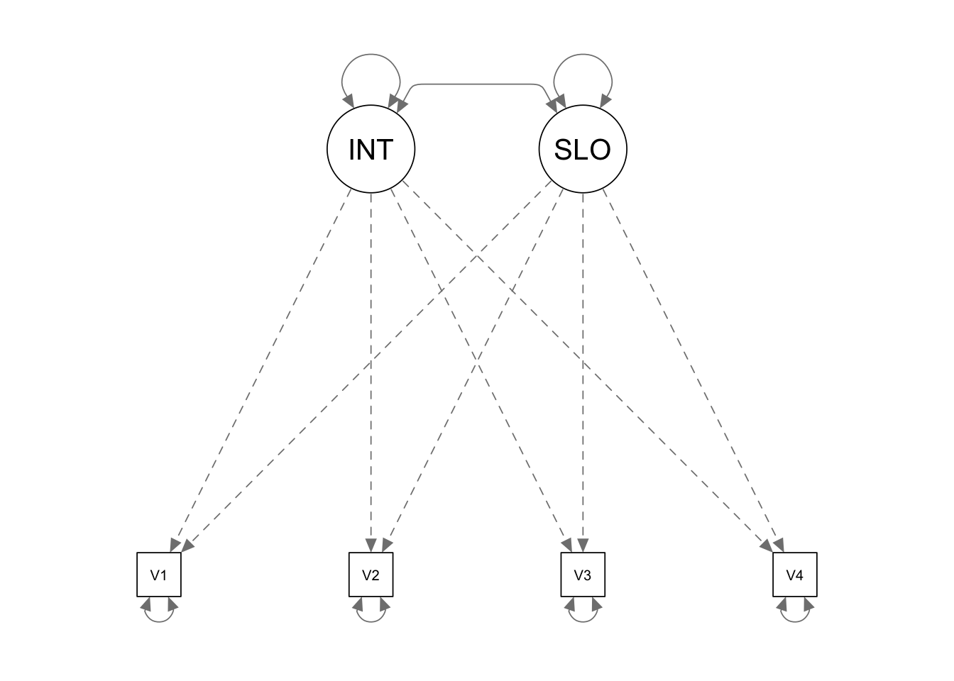
library(semPlot)Example: Power for LGM
In this example, we would like to conduct power analysis for a latent growth model.
Define the population model
We first use the lavaan model syntax to define our
population model and supply all the parameter values. To supply the
population value of a parameter, we just need to multiply the parameter
with the numeric value.
popmodel <- '

INTERC =~ 1*V1 + 1*V2 + 1*V3 + 1*V4
SLOPE =~ 0*V1 + 1*V2 + 2*V3 + 3*V4

INTERC ~~ 1*INTERC + -.10*SLOPE
SLOPE ~~ .04*SLOPE

INTERC ~ 5*1
SLOPE ~ .5*1

# error variance
V1 ~~ .25*V1
V2 ~~ .25*V2
V3 ~~ .25*V3
V4 ~~ .25*V4

# intercepts
V1 ~ 0*1
V2 ~ 0*1
V3 ~ 0*1
V4 ~ 0*1

'
Define the analysis model
Next we use the lavaan model syntax to define the
analysis model. This is the model syntax you would write as if you have
a data set at hand (we are very familiar with it already). The analysis
model does not necessarily have to be the same as the population
model.
Analyze.model <- '
INTERC =~ 1*V1 + 1*V2 + 1*V3 + 1*V4
SLOPE =~ 0*V1 + 1*V2 + 2*V3 + 3*V4

INTERC ~~ INTERC + SLOPE
SLOPE ~~ SLOPE


INTERC ~ 1
SLOPE ~ 1

V1 ~~ a*V1
V2 ~~ a*V2
V3 ~~ a*V3
V4 ~~ a*V4

V1 ~ 0*1
V2 ~ 0*1
V3 ~ 0*1
V4 ~ 0*1

'
Conduct power analysis
Last, we call up the sim() function available in the
simsem R package. This function will automatically generate
multiple copies of data based on the population model and fit the
analysis model to the simulated data. It will output the results
summarized over replications.
For this example, we request sim() to generate 1000
copies of data, each has a sample size of 303. We also request
sim() to use lavaan’s sem()
function when fitting the analysis model to the simulated data. For more
detailed information about the simsem package, please refer
to its webpage.
Output <- sim(1000, Analyze.model, n = 200, generate = popmodel, lavaanfun = "sem")summary(Output)## RESULT OBJECT
## Model Type
## [1] "lavaan"
## ========= Fit Indices Cutoffs ============
## Alpha
## Fit Indices 0.1 0.05 0.01 0.001 Mean SD
## chisq 9.116 11.144 14.342 18.761 4.916 3.108
## aic 1218.903 1229.157 1248.090 1268.953 1176.910 32.507
## bic 1244.711 1254.965 1273.898 1294.760 1202.717 32.507
## rmsea 0.080 0.097 0.120 0.146 0.024 0.035
## cfi 0.988 0.983 0.973 0.956 0.997 0.006
## tli 0.986 0.980 0.967 0.947 1.000 0.011
## srmr 0.052 0.060 0.073 0.086 0.034 0.014
## ========= Parameter Estimates and Standard Errors ============
## Estimate Average Estimate SD Average SE
## INTERC~~INTERC 0.985 0.152 0.147
## INTERC~~SLOPE -0.099 0.036 0.035
## SLOPE~~SLOPE 0.040 0.015 0.014
## INTERC~1 4.998 0.097 0.094
## SLOPE~1 0.500 0.026 0.026
## V1~~V1 0.249 0.068 0.066
## V2~~V2 0.251 0.043 0.043
## V3~~V3 0.249 0.042 0.042
## V4~~V4 0.253 0.066 0.063
## Power (Not equal 0) Std Est Std Est SD Std Ave SE
## INTERC~~INTERC 1.000 1.000 0.000 0.000
## INTERC~~SLOPE 0.833 -0.500 0.119 0.122
## SLOPE~~SLOPE 0.817 1.000 0.000 0.000
## INTERC~1 1.000 5.083 0.416 0.395
## SLOPE~1 1.000 2.677 0.664 0.654
## V1~~V1 0.978 0.203 0.057 0.054
## V2~~V2 1.000 0.234 0.040 0.039
## V3~~V3 1.000 0.251 0.041 0.041
## V4~~V4 0.990 0.253 0.063 0.062
## Average Param Average Bias Coverage
## INTERC~~INTERC 1.00 -0.015 0.939
## INTERC~~SLOPE -0.10 0.001 0.939
## SLOPE~~SLOPE 0.04 0.000 0.950
## INTERC~1 5.00 -0.002 0.932
## SLOPE~1 0.50 0.000 0.948
## V1~~V1 0.25 -0.001 0.943
## V2~~V2 0.25 0.001 0.955
## V3~~V3 0.25 -0.001 0.940
## V4~~V4 0.25 0.003 0.943
## ========= Correlation between Fit Indices ============
## chisq aic bic rmsea cfi tli srmr
## chisq 1.000 0.077 0.077 0.946 -0.913 -0.993 0.788
## aic 0.077 1.000 1.000 0.063 -0.048 -0.079 0.074
## bic 0.077 1.000 1.000 0.063 -0.048 -0.079 0.074
## rmsea 0.946 0.063 0.063 1.000 -0.932 -0.938 0.729
## cfi -0.913 -0.048 -0.048 -0.932 1.000 0.918 -0.668
## tli -0.993 -0.079 -0.079 -0.938 0.918 1.000 -0.787
## srmr 0.788 0.074 0.074 0.729 -0.668 -0.787 1.000
## ================== Replications =====================
## Number of replications = 1000
## Number of converged replications = 998
## Number of nonconverged replications:
## 1. Nonconvergent Results = 0
## 2. Nonconvergent results from multiple imputation = 0
## 3. At least one SE were negative or NA = 0
## 4. Nonpositive-definite latent or observed (residual) covariance matrix
## (e.g., Heywood case or linear dependency) = 2Example: Power with MCAR missing data
We are using the same population model and analysis model as above.
define missing data template
Missing data template can be defined using the miss
function in simsem. The pmMCAR argument
indicates the proportion of values in each variable that will be missing
completely at random.
missmodel <- miss(pmMCAR = 0.2)Conduct power analysis
The missing data template can be incorporated in the simulation
process with the miss = argument.
Output <- sim(1000, Analyze.model, n = 200, generate = popmodel, lavaanfun = "sem", miss = missmodel)summary(Output)## RESULT OBJECT
## Model Type
## [1] "lavaan"
## ========= Fit Indices Cutoffs ============
## Alpha
## Fit Indices 0.1 0.05 0.01 0.001 Mean SD
## chisq 9.197 11.061 16.038 19.954 5.128 3.248
## aic 1857.108 1871.257 1895.818 1933.618 1806.467 40.690
## bic 1886.793 1900.942 1925.503 1963.303 1836.152 40.690
## rmsea 0.065 0.078 0.105 0.122 0.021 0.029
## cfi 0.992 0.989 0.979 0.976 0.998 0.004
## tli 0.990 0.987 0.974 0.971 1.000 0.007
## srmr 0.044 0.048 0.056 0.067 0.028 0.011
## ========= Parameter Estimates and Standard Errors ============
## Estimate Average Estimate SD Average SE
## INTERC~~INTERC 0.989 0.123 0.119
## INTERC~~SLOPE -0.099 0.030 0.029
## SLOPE~~SLOPE 0.040 0.012 0.012
## INTERC~1 5.000 0.077 0.076
## SLOPE~1 0.500 0.022 0.021
## V1~~V1 0.249 0.054 0.054
## V2~~V2 0.251 0.036 0.035
## V3~~V3 0.252 0.034 0.034
## V4~~V4 0.248 0.053 0.050
## Power (Not equal 0) Std Est Std Est SD Std Ave SE
## INTERC~~INTERC 1.000 1.000 0.000 0.000
## INTERC~~SLOPE 0.959 -0.498 0.093 0.091
## SLOPE~~SLOPE 0.949 1.000 0.000 0.000
## INTERC~1 1.000 5.057 0.325 0.316
## SLOPE~1 1.000 2.599 0.482 0.454
## V1~~V1 0.999 0.202 0.044 0.043
## V2~~V2 1.000 0.233 0.032 0.032
## V3~~V3 1.000 0.252 0.034 0.033
## V4~~V4 1.000 0.248 0.050 0.050
## Average Param Average Bias Coverage
## INTERC~~INTERC 1.00 -0.011 0.930
## INTERC~~SLOPE -0.10 0.001 0.943
## SLOPE~~SLOPE 0.04 0.000 0.947
## INTERC~1 5.00 0.000 0.941
## SLOPE~1 0.50 0.000 0.935
## V1~~V1 0.25 -0.001 0.944
## V2~~V2 0.25 0.001 0.946
## V3~~V3 0.25 0.002 0.951
## V4~~V4 0.25 -0.002 0.935
## ========= Correlation between Fit Indices ============
## chisq aic bic rmsea cfi tli srmr
## chisq 1.000 0.032 0.032 0.944 -0.925 -0.995 0.791
## aic 0.032 1.000 1.000 0.033 -0.035 -0.029 0.028
## bic 0.032 1.000 1.000 0.033 -0.035 -0.029 0.028
## rmsea 0.944 0.033 0.033 1.000 -0.935 -0.941 0.730
## cfi -0.925 -0.035 -0.035 -0.935 1.000 0.923 -0.675
## tli -0.995 -0.029 -0.029 -0.941 0.923 1.000 -0.791
## srmr 0.791 0.028 0.028 0.730 -0.675 -0.791 1.000
## ================== Replications =====================
## Number of replications = 1000
## Number of converged replications = 1000
## Number of nonconverged replications:
## 1. Nonconvergent Results = 0
## 2. Nonconvergent results from multiple imputation = 0
## 3. At least one SE were negative or NA = 0
## 4. Nonpositive-definite latent or observed (residual) covariance matrix
## (e.g., Heywood case or linear dependency) = 0Example: Power with attrition
We are using the same population model and analysis model as above.
Define missing data template
Missing data template can be defined using the miss
function in simsem. The prAttr argument
indicates the probability of an entire case being removed due to
attrition at each time point. Note that the probability is computed out
of the remaining case at the each time point.
missmodel <- miss(prAttr = c(0, 0.2, 1/4, 1/3), timePoints = 4)Conduct power analysis
Output <- sim(10000, Analyze.model, n = 130, generate = popmodel, lavaanfun = "sem", miss = missmodel, seed = 10011, multicore = T)summary(Output)## RESULT OBJECT
## Model Type
## [1] "lavaan"
## ========= Fit Indices Cutoffs ============
## Alpha
## Fit Indices 0.1 0.05 0.01 0.001 Mean SD
## chisq 13.895 16.160 20.842 27.012 8.359 4.189
## aic 917.215 931.075 956.364 985.774 867.983 38.273
## bic 934.421 948.281 973.569 1002.979 885.189 38.273
## rmsea 0.075 0.089 0.111 0.135 0.026 0.033
## cfi 0.972 0.961 0.940 0.904 0.992 0.014
## tli 0.979 0.971 0.955 0.928 0.999 0.015
## srmr 0.085 0.097 0.122 0.156 0.056 0.022
## ========= Parameter Estimates and Standard Errors ============
## Estimate Average Estimate SD Average SE
## INTERC~~INTERC 0.990 0.150 0.149
## INTERC~~SLOPE -0.099 0.042 0.042
## SLOPE~~SLOPE 0.039 0.018 0.017
## INTERC~1 5.000 0.096 0.095
## SLOPE~1 0.500 0.035 0.034
## a <- (V1~~V1) 0.250 0.029 0.029
## a <- (V2~~V2) 0.250 0.029 0.029
## a <- (V3~~V3) 0.250 0.029 0.029
## a <- (V4~~V4) 0.250 0.029 0.029
## [ a ] - [ a ] # 1 0.000 0.000 NA
## [ a ] - [ a ] # 2 0.000 0.000 NA
## [ a ] - [ a ] # 3 0.000 0.000 NA
## Power (Not equal 0) Std Est Std Est SD Std Ave SE
## INTERC~~INTERC 1.000 1.000 0.000 0.000
## INTERC~~SLOPE 0.680 -0.512 0.208 0.407
## SLOPE~~SLOPE 0.635 1.000 0.000 0.000
## INTERC~1 1.000 5.069 0.405 0.397
## SLOPE~1 1.000 2.827 1.344 1.899
## a <- (V1~~V1) 1.000 0.205 0.033 0.033
## a <- (V2~~V2) 1.000 0.234 0.034 0.034
## a <- (V3~~V3) 1.000 0.253 0.040 0.039
## a <- (V4~~V4) 1.000 0.256 0.050 0.049
## [ a ] - [ a ] # 1 1.000 -0.029 0.013 0.013
## [ a ] - [ a ] # 2 1.000 -0.048 0.028 0.027
## [ a ] - [ a ] # 3 1.000 -0.052 0.043 0.042
## Average FMI1 SD FMI1
## INTERC~~INTERC 0.038 0.180
## INTERC~~SLOPE -0.283 24.592
## SLOPE~~SLOPE 0.423 4.643
## INTERC~1 0.018 0.017
## SLOPE~1 0.338 0.837
## a <- (V1~~V1) 0.405 0.057
## a <- (V2~~V2) 0.405 0.057
## a <- (V3~~V3) 0.405 0.057
## a <- (V4~~V4) 0.405 0.057
## [ a ] - [ a ] # 1 NaN NA
## [ a ] - [ a ] # 2 NaN NA
## [ a ] - [ a ] # 3 NaN NA
## ========= Correlation between Fit Indices ============
## chisq aic bic rmsea cfi tli srmr
## chisq 1.000 0.015 0.015 0.943 -0.911 -0.987 0.645
## aic 0.015 1.000 1.000 0.012 0.014 -0.014 -0.067
## bic 0.015 1.000 1.000 0.012 0.014 -0.014 -0.067
## rmsea 0.943 0.012 0.012 1.000 -0.929 -0.930 0.590
## cfi -0.911 0.014 0.014 -0.929 1.000 0.913 -0.582
## tli -0.987 -0.014 -0.014 -0.930 0.913 1.000 -0.650
## srmr 0.645 -0.067 -0.067 0.590 -0.582 -0.650 1.000
## ================== Replications =====================
## Number of replications = 10000
## Number of converged replications = 9867
## Number of nonconverged replications:
## 1. Nonconvergent Results = 0
## 2. Nonconvergent results from multiple imputation = 0
## 3. At least one SE were negative or NA = 0
## 4. Nonpositive-definite latent or observed (residual) covariance matrix
## (e.g., Heywood case or linear dependency) = 133
## NOTE: The data generation model is not the same as the analysis model. See the summary of the population underlying data generation by the summaryPopulation function.Example: Power with Planned Missing Data
Define missing data patterns
# Define the missing data patterns using a logical matrix

miss.mat <- matrix(0, nrow = 200, ncol = 4)

miss.row1 <- sample(1:nrow(miss.mat), 100, replace = F)

miss.mat[miss.row1, 1] <- 1
miss.mat[setdiff(1:nrow(miss.mat), miss.row1), 4] <- 1

# create the missing data template
missmodel <- miss(logical = apply(miss.mat, 2, as.logical), m = 0)
Conduct Power Analysis
Output <- sim(1000, Analyze.model, n = 200, generate = popmodel, lavaanfun = "sem", miss = missmodel, seed = 10291, multicore = T)summary(Output)## RESULT OBJECT
## Model Type
## [1] "lavaan"
## ========= Fit Indices Cutoffs ============
## Alpha
## Fit Indices 0.1 0.05 0.01 0.001 Mean SD
## chisq 11.778 13.597 17.102 22.139 6.968 3.621
## aic 1445.144 1459.544 1479.277 1496.805 1401.684 35.370
## bic 1464.934 1479.334 1499.067 1516.595 1421.474 35.370
## rmsea 0.049 0.059 0.075 0.094 0.014 0.021
## cfi 0.989 0.984 0.971 0.955 0.997 0.006
## tli 0.992 0.988 0.979 0.966 1.002 0.008
## srmr 0.069 0.080 0.095 0.124 0.047 0.017
## ========= Parameter Estimates and Standard Errors ============
## Estimate Average Estimate SD Average SE
## INTERC~~INTERC 0.992 0.139 0.138
## INTERC~~SLOPE -0.099 0.041 0.042
## SLOPE~~SLOPE 0.040 0.020 0.020
## INTERC~1 5.000 0.080 0.082
## SLOPE~1 0.500 0.028 0.028
## a <- (V1~~V1) 0.249 0.024 0.024
## a <- (V2~~V2) 0.249 0.024 0.024
## a <- (V3~~V3) 0.249 0.024 0.024
## a <- (V4~~V4) 0.249 0.024 0.024
## [ a ] - [ a ] # 1 0.000 0.000 NA
## [ a ] - [ a ] # 2 0.000 0.000 NA
## [ a ] - [ a ] # 3 0.000 0.000 NA
## Power (Not equal 0) Std Est Std Est SD Std Ave SE
## INTERC~~INTERC 1.000 1.000 0.000 0.000
## INTERC~~SLOPE 0.663 -0.516 0.236 0.463
## SLOPE~~SLOPE 0.537 1.000 0.000 0.000
## INTERC~1 1.000 5.058 0.370 0.366
## SLOPE~1 1.000 2.895 1.877 3.895
## a <- (V1~~V1) 1.000 0.203 0.031 0.031
## a <- (V2~~V2) 1.000 0.232 0.028 0.028
## a <- (V3~~V3) 1.000 0.250 0.031 0.030
## a <- (V4~~V4) 1.000 0.251 0.041 0.038
## [ a ] - [ a ] # 1 1.000 -0.028 0.011 0.010
## [ a ] - [ a ] # 2 1.000 -0.046 0.022 0.021
## [ a ] - [ a ] # 3 1.000 -0.048 0.035 0.033
## Average FMI1 SD FMI1
## INTERC~~INTERC 0.276 0.232
## INTERC~~SLOPE -0.794 22.915
## SLOPE~~SLOPE 0.417 10.031
## INTERC~1 0.138 0.022
## SLOPE~1 0.289 1.063
## a <- (V1~~V1) 0.396 0.064
## a <- (V2~~V2) 0.396 0.064
## a <- (V3~~V3) 0.396 0.064
## a <- (V4~~V4) 0.396 0.064
## [ a ] - [ a ] # 1 NaN NA
## [ a ] - [ a ] # 2 NaN NA
## [ a ] - [ a ] # 3 NaN NA
## ========= Correlation between Fit Indices ============
## chisq aic bic rmsea cfi tli srmr
## chisq 1.000 -0.004 -0.004 0.905 -0.848 -0.992 0.601
## aic -0.004 1.000 1.000 -0.020 0.026 0.005 -0.031
## bic -0.004 1.000 1.000 -0.020 0.026 0.005 -0.031
## rmsea 0.905 -0.020 -0.020 1.000 -0.927 -0.896 0.526
## cfi -0.848 0.026 0.026 -0.927 1.000 0.853 -0.519
## tli -0.992 0.005 0.005 -0.896 0.853 1.000 -0.596
## srmr 0.601 -0.031 -0.031 0.526 -0.519 -0.596 1.000
## ================== Replications =====================
## Number of replications = 1000
## Number of converged replications = 969
## Number of nonconverged replications:
## 1. Nonconvergent Results = 1
## 2. Nonconvergent results from multiple imputation = 0
## 3. At least one SE were negative or NA = 0
## 4. Nonpositive-definite latent or observed (residual) covariance matrix
## (e.g., Heywood case or linear dependency) = 30
## NOTE: The data generation model is not the same as the analysis model. See the summary of the population underlying data generation by the summaryPopulation function.© Copyright 2024 @Yi Feng and @Gregory R. Hancock.