EDMS 657-R Tutorial: Tree-based Methods
Yi Feng
EDMS, University of MarylandFirst, let’s load all the required packages.
install.packages("tree")
install.packages("randomForest")
install.packages("rpart")
install.packages("caret")
install.packages("rpart.plot")
install.packages("gbm")
library(tree)
library(randomForest)
library(rpart)
library(caret)
library(rpart.plot)
library(gbm)
library(EDMS657Data)
Regression Trees
We will use the Major League Baseball Data for the demonstration of regression trees. In this example, we are interested in predicting the log-transformed salary.
We first fit the regression tree to a subset of the baseball data, predicting the log transformed salary.
data("hitters")

# log transform the salary
hitters$lgSalary <- log(hitters$Salary)

# you can use the tree package
tree.hitters <- tree(lgSalary ~., hitters[is.na(hitters$Salary) == F, c("lgSalary","Years","Hits")])
summary(tree.hitters)
##
## Regression tree:
## tree(formula = lgSalary ~ ., data = hitters[is.na(hitters$Salary) ==
## F, c("lgSalary", "Years", "Hits")])
## Number of terminal nodes: 8
## Residual mean deviance: 0.2708 = 69.06 / 255
## Distribution of residuals:
## Min. 1st Qu. Median Mean 3rd Qu. Max.
## -2.2400 -0.2980 -0.0365 0.0000 0.3233 2.1520# you can also use the rpart package
tree.hitters_2 <- rpart(formula = lgSalary ~.,
data = hitters[is.na(hitters$Salary) == F, c("lgSalary","Years","Hits")],
method = "anova",
control = list(cp = 0.005))
tree.hitters_2## n= 263
##
## node), split, n, deviance, yval
## * denotes terminal node
##
## 1) root 263 207.153700 5.927222
## 2) Years< 4.5 90 42.353170 5.106790
## 4) Years< 3.5 62 23.008670 4.891812
## 8) Hits< 114 43 17.145680 4.727386
## 16) Hits>=42 36 3.098678 4.637745 *
## 17) Hits< 42 7 12.269990 5.188399 *
## 9) Hits>=114 19 2.069451 5.263932 *
## 5) Years>=3.5 28 10.134390 5.582812
## 10) Hits< 106 14 1.791944 5.315652 *
## 11) Hits>=106 14 6.343952 5.849973 *
## 3) Years>=4.5 173 72.705310 6.354036
## 6) Hits< 117.5 90 28.093710 5.998380
## 12) Years< 6.5 26 7.237690 5.688925 *
## 13) Years>=6.5 64 17.354710 6.124096
## 26) Hits< 50.5 12 2.689439 5.730017 *
## 27) Hits>=50.5 52 12.371640 6.215037 *
## 7) Hits>=117.5 83 20.883070 6.739687 *we can plot the regression tree.
# if you are using the tree package
plot(tree.hitters)
text(tree.hitters, pretty = 0)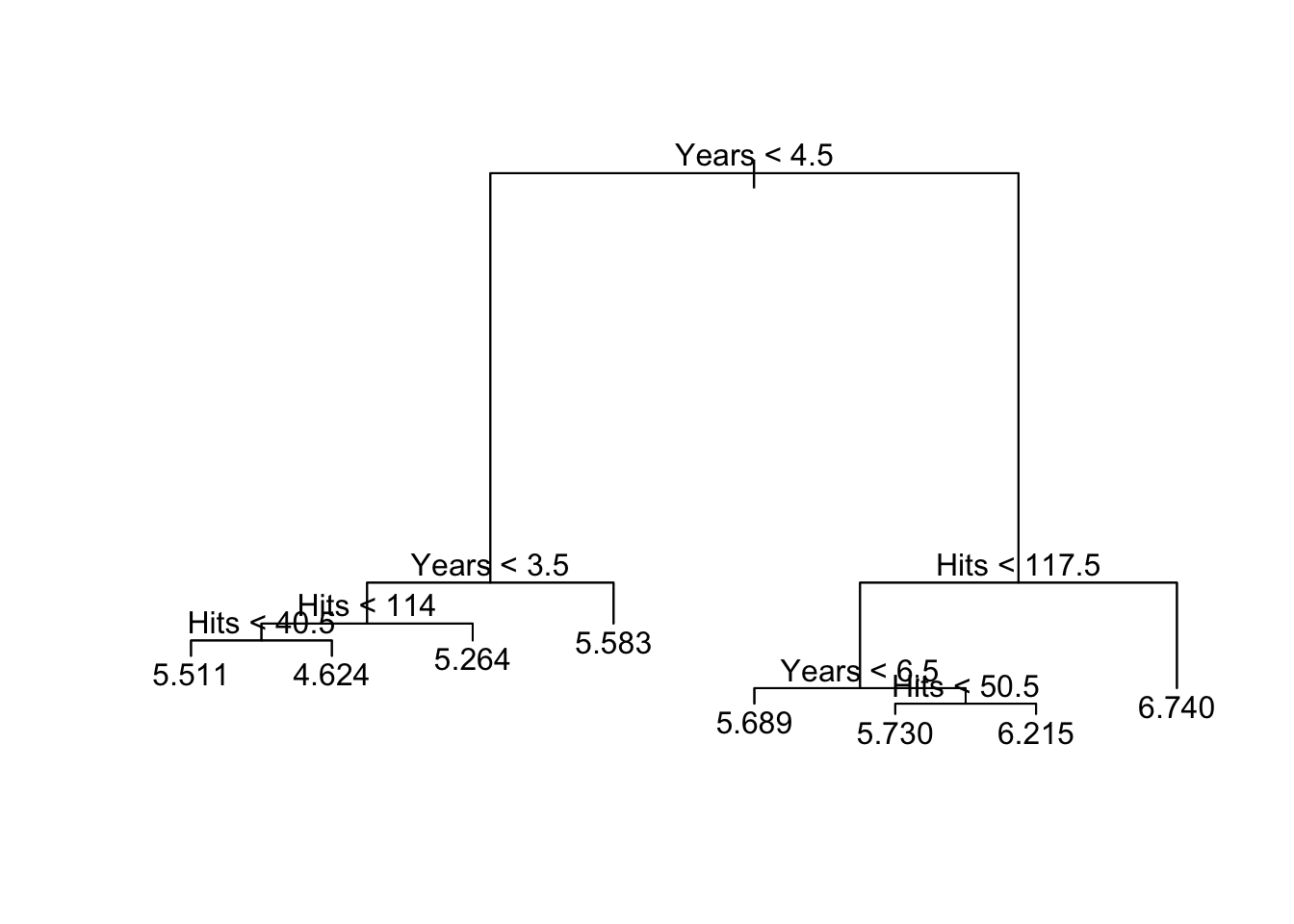
# if you are using the rpart package
rpart.plot(tree.hitters_2)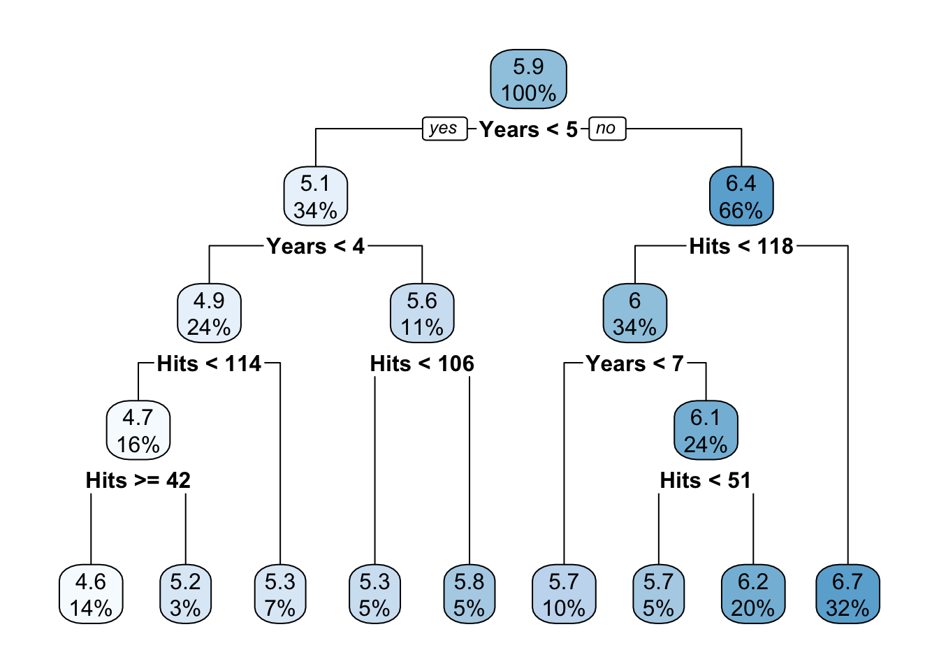
To avoid over-fitting, we should consider pruning the tree. Here we try to only keep 3 terminal nodes.
# if using the tree package
prune.hitters <- prune.tree(tree.hitters, best = 3)

summary(prune.hitters)
##
## Regression tree:
## snip.tree(tree = tree.hitters, nodes = c(6L, 2L))
## Number of terminal nodes: 3
## Residual mean deviance: 0.3513 = 91.33 / 260
## Distribution of residuals:
## Min. 1st Qu. Median Mean 3rd Qu. Max.
## -2.24000 -0.39580 -0.03162 0.00000 0.33380 2.55600plot(prune.hitters)
text(prune.hitters)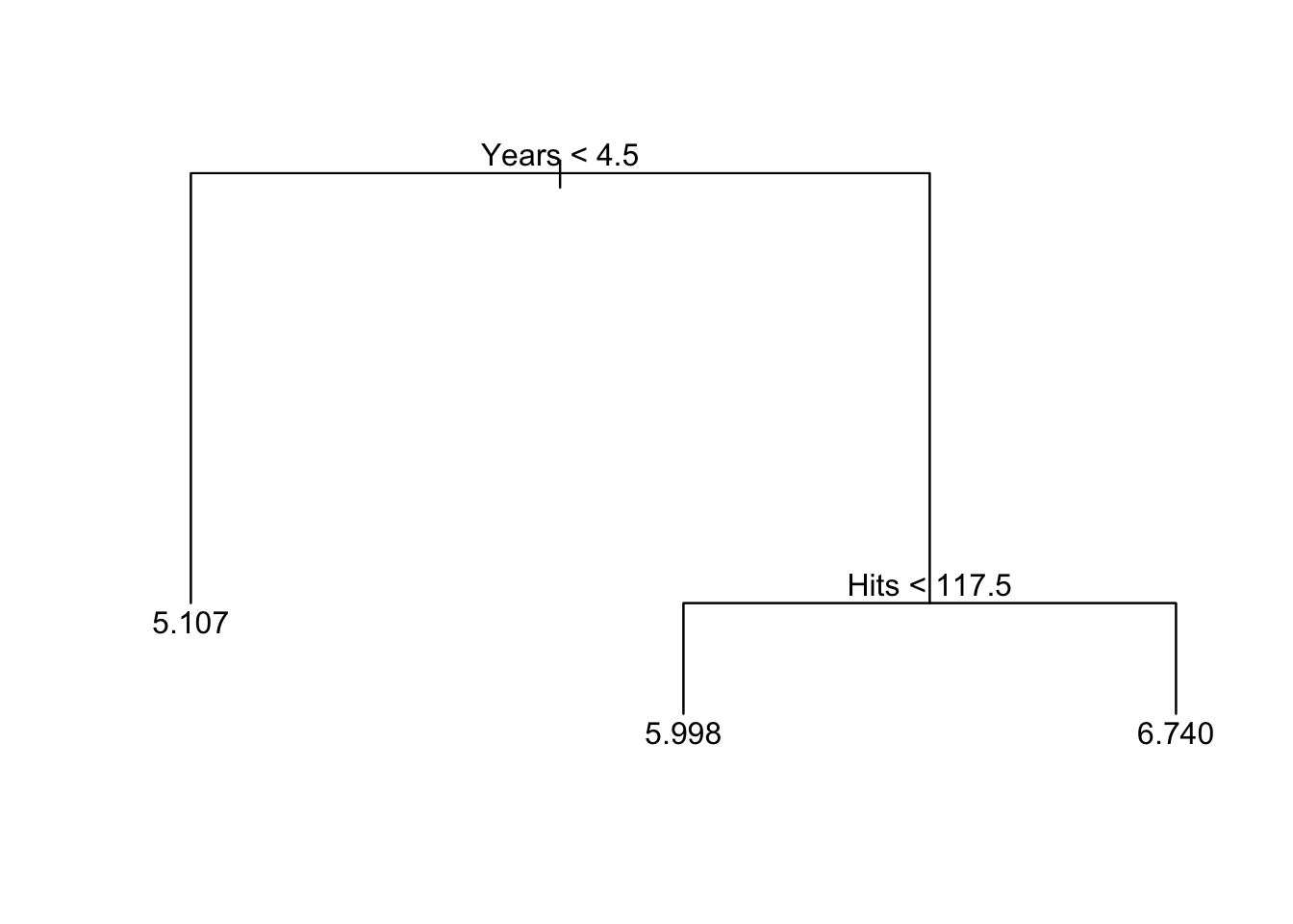
# if using the rpart package
prune.hitters_2 <- rpart(formula = lgSalary ~.,
  data = hitters[is.na(hitters$Salary) == F, c("lgSalary","Years","Hits")],
  method = "anova",
  control = list(cp = 0.1))

prune.hitters_2
## n= 263
##
## node), split, n, deviance, yval
## * denotes terminal node
##
## 1) root 263 207.15370 5.927222
## 2) Years< 4.5 90 42.35317 5.106790 *
## 3) Years>=4.5 173 72.70531 6.354036
## 6) Hits< 117.5 90 28.09371 5.998380 *
## 7) Hits>=117.5 83 20.88307 6.739687 *rpart.plot(prune.hitters_2)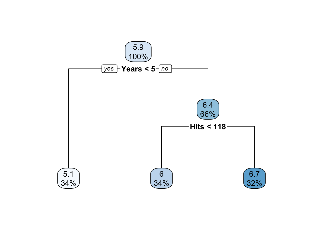
Cost Complexity Pruning
The cost complexity parameter is a tuning parameter for which we need to seek an optimal value through cross-validation.
hitters2 <- hitters[is.na(hitters$Salary)==F, c("lgSalary","Years","Hits","HmRun","RBI","PutOuts","Walks","Runs")]

set.seed(123)
train <- sample(1:nrow(hitters2), 132, replace=F)

# if using the tree package
tree2.hitters <- tree(lgSalary~., hitters2[train,])
summary(tree2.hitters)
##
## Regression tree:
## tree(formula = lgSalary ~ ., data = hitters2[train, ])
## Variables actually used in tree construction:
## [1] "Years" "Hits" "Runs" "Walks" "RBI"
## Number of terminal nodes: 10
## Residual mean deviance: 0.1857 = 22.65 / 122
## Distribution of residuals:
## Min. 1st Qu. Median Mean 3rd Qu. Max.
## -1.555000 -0.202200 0.004768 0.000000 0.237100 1.156000plot(tree2.hitters)
text(tree2.hitters, pretty = 0)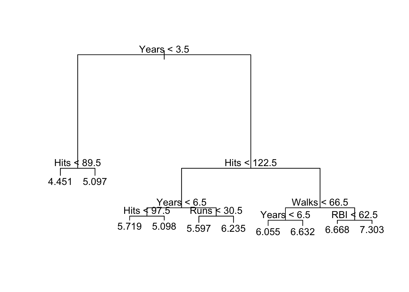
# pruning the tree via cross-validation
cv.tree2 <- cv.tree(tree2.hitters, K = 10)
plot(cv.tree2$size,cv.tree2$dev, type = "b")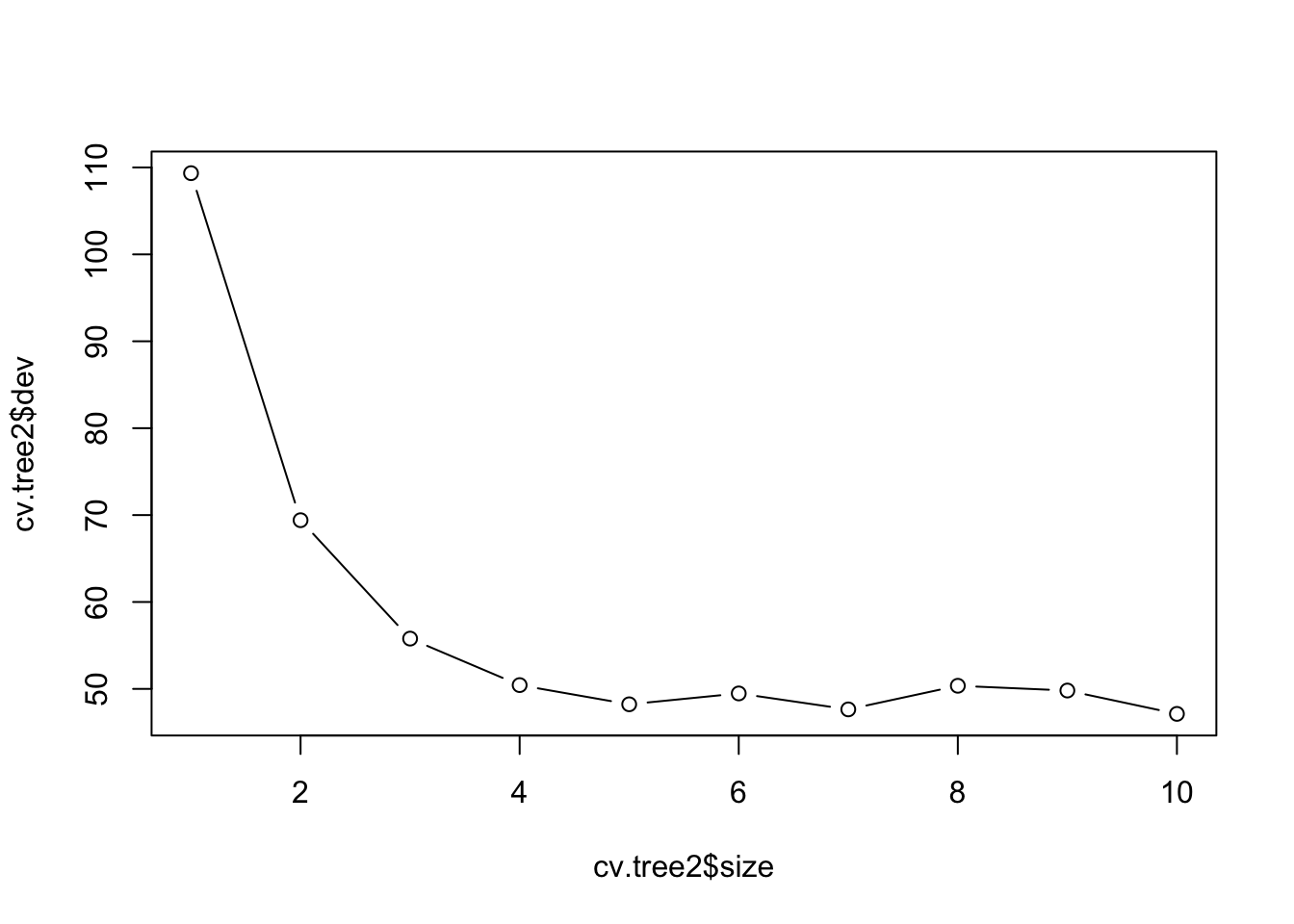
# if using the rpart package

tree2.hitters_2 <- rpart(formula = lgSalary ~.,
  data = hitters2[train,],
  method = "anova",
  control = list(cp = 0, xval = 10))   #10-fold cv

plotcp(tree2.hitters_2)  # A good choice of cp for pruning is often the leftmost value for which the mean lies below the horizontal line.
abline(v = 6, lty = "dashed")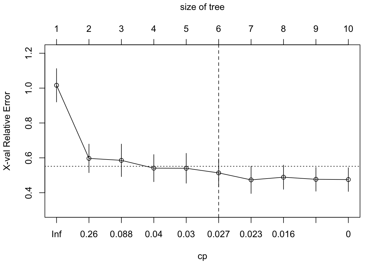
The cross-validation results suggest that we should keep four
terminal nodes using the tree package and 6 terminal nodes
using the rpart package.
# if using the tree package
prune.hitters2 <- prune.tree(tree2.hitters, best = 4)
plot(prune.hitters2)
text(prune.hitters2)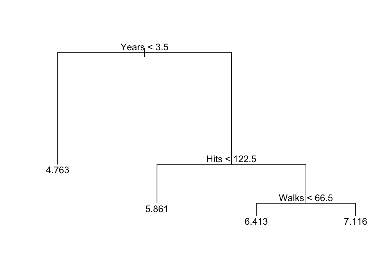
# if using the rpart package
prune.hitters2_2 <- rpart(formula = lgSalary ~.,
  data = hitters2[train,],
  method = "anova",
  control = list(cp = 0.027))

rpart.plot(prune.hitters2_2)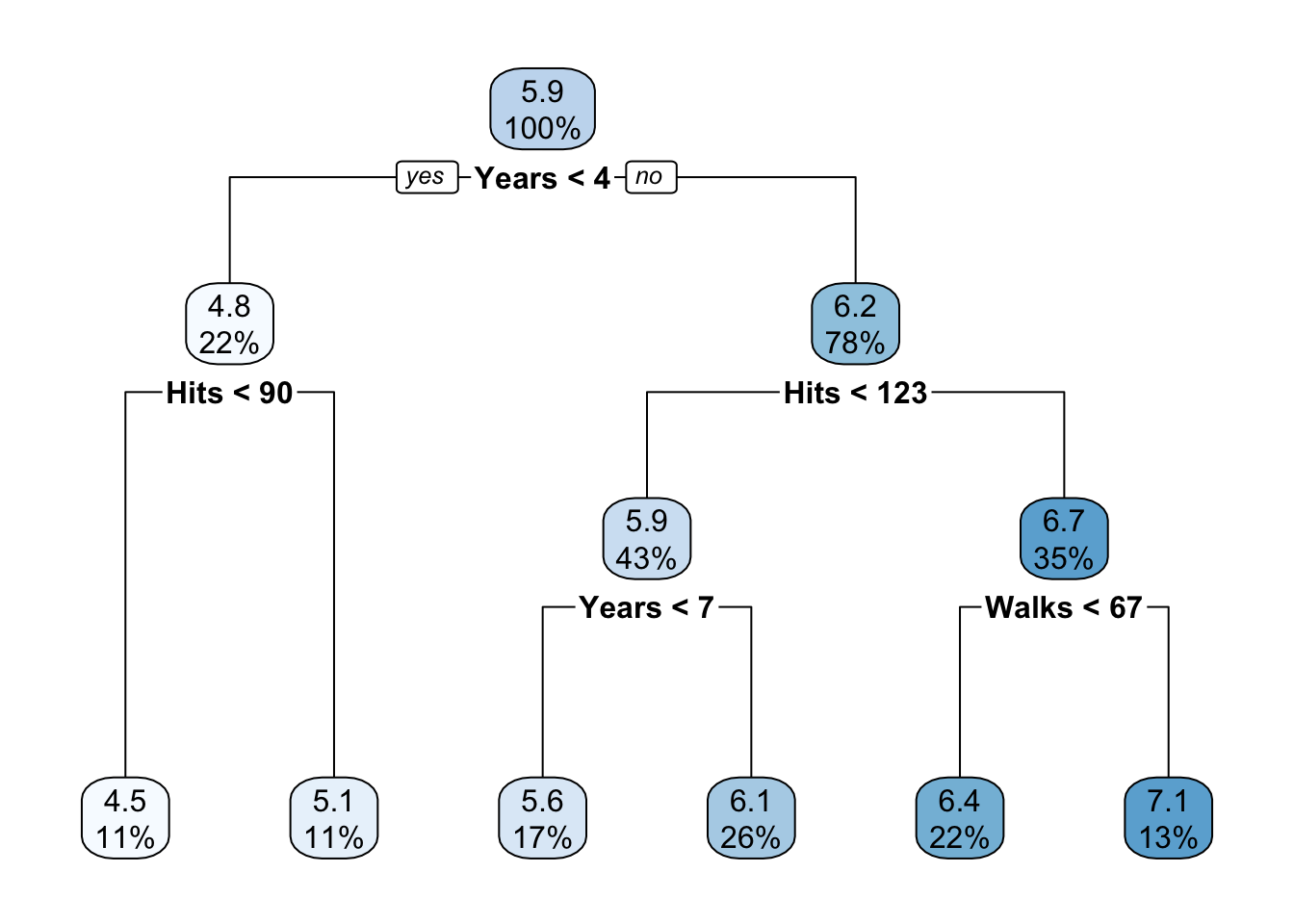
Classification Trees
In this example, we will use the patients’ data that contain a binary outcome HD for 303 patients who presented with chest pain. An outcome value of Yes indicates the presence of heart disease based on an angiographic test, while No means no heart disease. There are 13 predictors including Age, Sex, Chol (a cholesterol measurement), and other heart and lung function measurements such as Thal (Thallium stress test) and ChestPain symptoms.
We first fit a classification tree to the training data.
data("heart")

set.seed(1234)
train <- sample(1:nrow(heart), 150)

# if using the tree package
tree.heart <- tree(AHD ~ ., heart[train, ])
plot(tree.heart)
text(tree.heart, pretty = 0)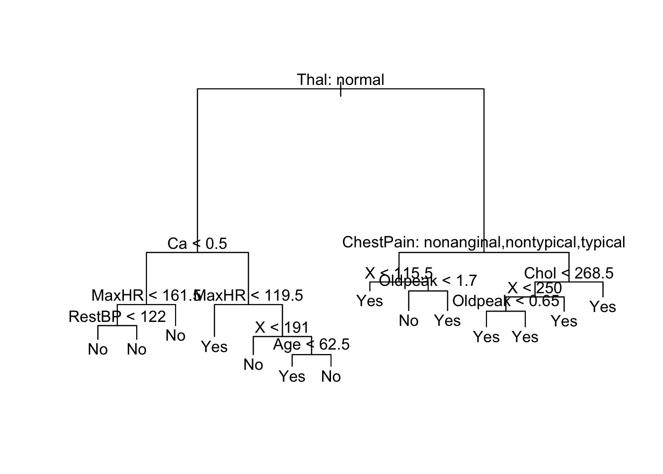
summary(tree.heart)##
## Classification tree:
## tree(formula = AHD ~ ., data = heart[train, ])
## Variables actually used in tree construction:
## [1] "Thal" "Ca" "MaxHR" "RestBP" "X"
## [6] "Age" "ChestPain" "Oldpeak" "Chol"
## Number of terminal nodes: 14
## Residual mean deviance: 0.4881 = 64.92 / 133
## Misclassification error rate: 0.102 = 15 / 147# if using the rpart package
tree.heart_2 <- rpart(AHD ~ ., heart[train, ],
method = "class",
control = list(minsplit = 0, cp = 0, xval = 0))
tree.heart_2## n= 150
##
## node), split, n, loss, yval, (yprob)
## * denotes terminal node
##
## 1) root 150 70 No (0.53333333 0.46666667)
## 2) Thal=normal 80 15 No (0.81250000 0.18750000)
## 4) Ca< 0.5 58 4 No (0.93103448 0.06896552) *
## 5) Ca>=0.5 22 11 No (0.50000000 0.50000000)
## 10) ChestPain=nonanginal,nontypical 9 1 No (0.88888889 0.11111111) *
## 11) ChestPain=asymptomatic,typical 13 3 Yes (0.23076923 0.76923077) *
## 3) Thal=fixed,reversable 70 15 Yes (0.21428571 0.78571429)
## 6) ChestPain=nonanginal,nontypical,typical 22 10 Yes (0.45454545 0.54545455)
## 12) Ca< 0.5 14 6 No (0.57142857 0.42857143)
## 24) X>=148 7 2 No (0.71428571 0.28571429) *
## 25) X< 148 7 3 Yes (0.42857143 0.57142857) *
## 13) Ca>=0.5 8 2 Yes (0.25000000 0.75000000) *
## 7) ChestPain=asymptomatic 48 5 Yes (0.10416667 0.89583333) *rpart.plot(tree.heart_2)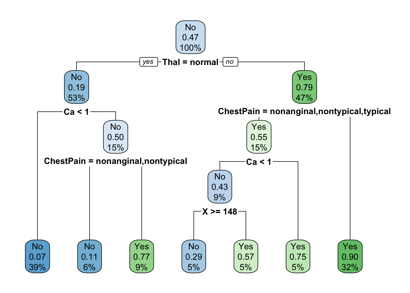
Next we proceed to cross-validation to prune the classifications
tree.You could use different criterion for pruning by specifying the
method = argument when using the tree
package.
cv.heart <- cv.tree(tree.heart)
plot(cv.heart$size, cv.heart$dev, type = "b")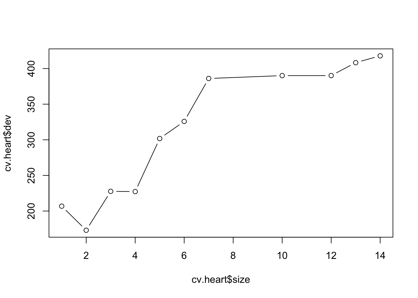
cv.heart <- cv.tree(tree.heart, method = "misclass")
plot(cv.heart$size,cv.heart$dev, type = "b")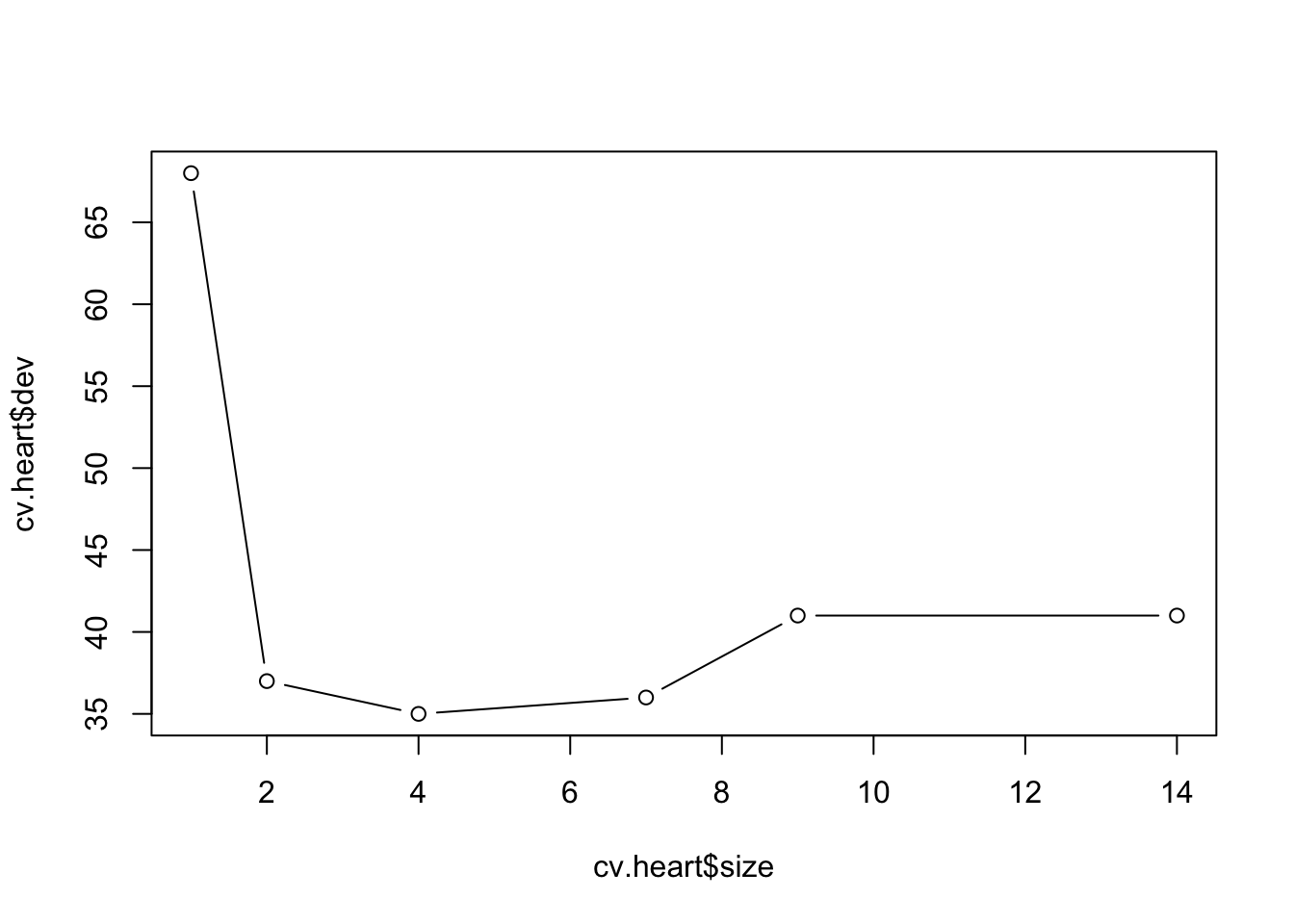
prune.heart <- prune.tree(tree.heart, best = 2)
plot(prune.heart)
text(prune.heart,pretty=0)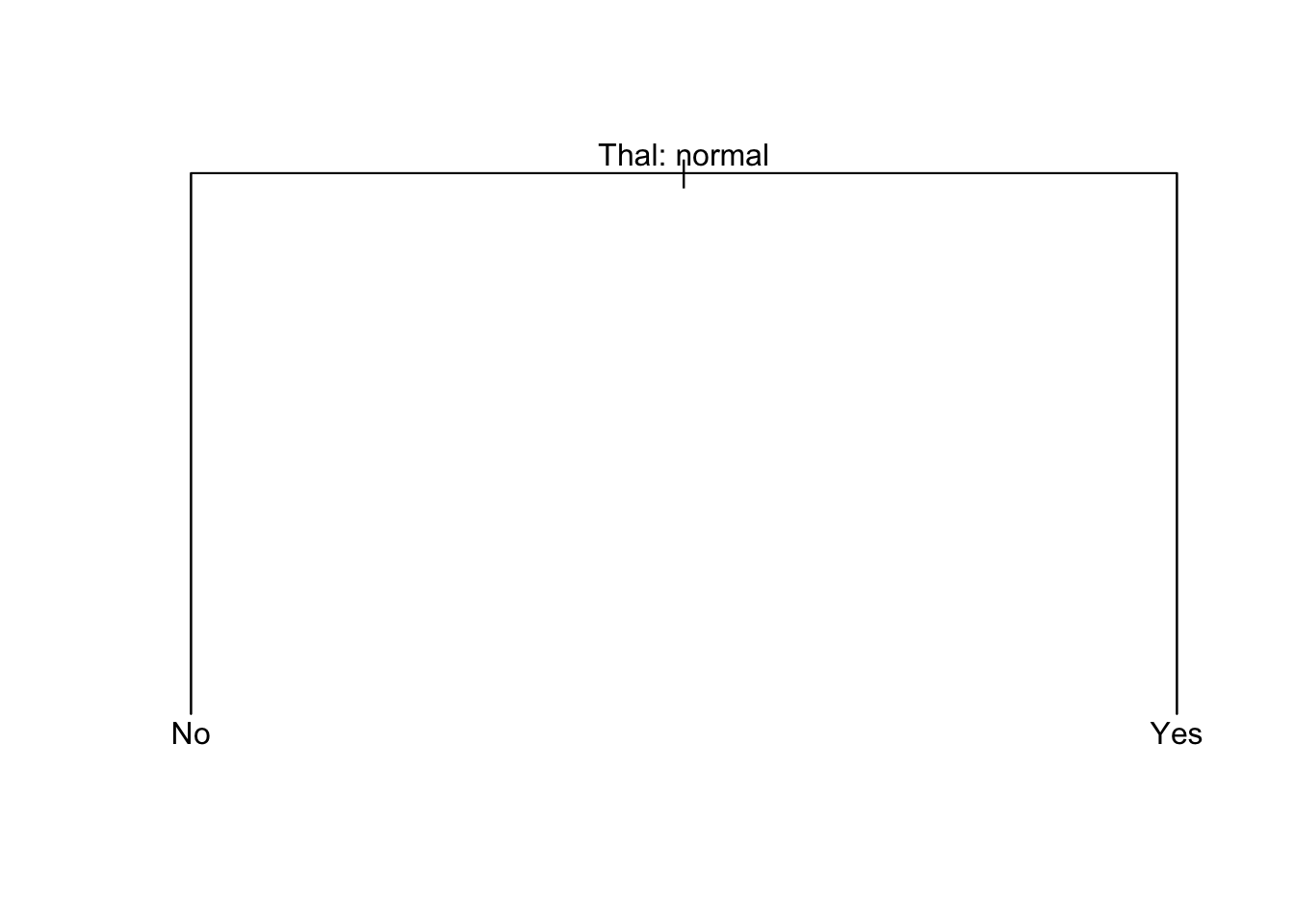
# if using the rpart package
cv.heart_2 <- rpart(AHD ~ ., heart[train, ],
  method = "class",
  control = list(cp = 0, xval = 10))
plotcp(cv.heart_2)
abline(v = 2, lty = "dashed")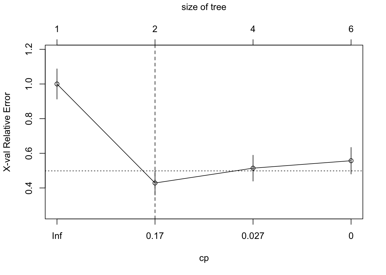
prune.heart_2 <- rpart(AHD ~ ., heart[train, ],
  method = "class",
  control = list(cp = 0.17))
rpart.plot(prune.heart_2)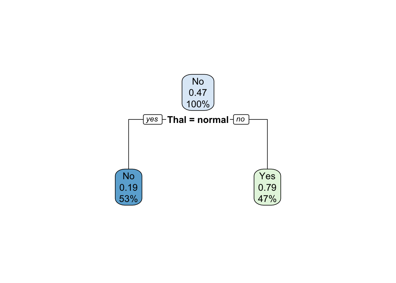
Bagging
Bagging is a special case of random forest. Therefore, we could use
the randomForest package to implement bagging. But you have
to specify mtry= to be the total number of predictors in
the original data. Here we use the baseball data as an example.
set.seed(234)
train <- sample(1:nrow(hitters2), 132, replace=F)

(bg.hitters <- randomForest(lgSalary~., data=hitters2, subset=train, mtry=7, importance=T))
##
## Call:
## randomForest(formula = lgSalary ~ ., data = hitters2, mtry = 7, importance = T, subset = train)
## Type of random forest: regression
## Number of trees: 500
## No. of variables tried at each split: 7
##
## Mean of squared residuals: 0.2571571
## % Var explained: 67.6Random Forest
We could implement random forest by changing the number of predictors
to be sampled at each split (mtry=). Here we use the
baseball data as an example.
(rf.hitters <- randomForest(lgSalary~., data=hitters2, subset=train, mtry=3, importance=T))##
## Call:
## randomForest(formula = lgSalary ~ ., data = hitters2, mtry = 3, importance = T, subset = train)
## Type of random forest: regression
## Number of trees: 500
## No. of variables tried at each split: 3
##
## Mean of squared residuals: 0.2407523
## % Var explained: 69.66Variable Importance Measures
imp.hitters <- importance(rf.hitters)

imp.hitters <- imp.hitters[order(imp.hitters[,2], decreasing=T),]
barplot(imp.hitters[,2], names.arg=rownames(imp.hitters), main="Variable importance", col="darkred", horiz=TRUE,las=1)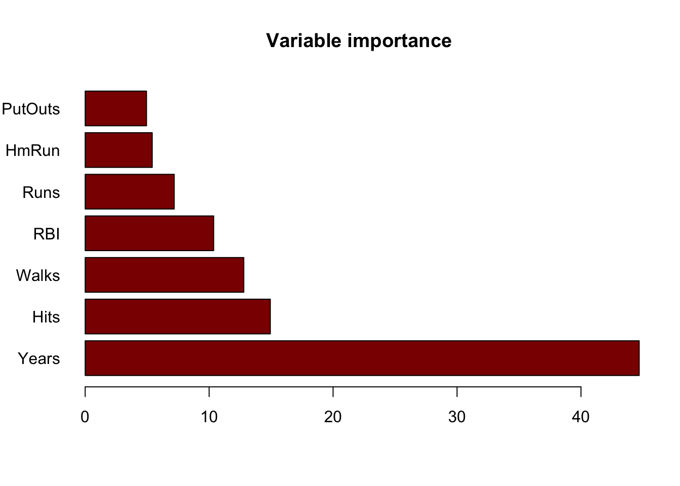
Boosting
We could use the gbm package to implement boosting. The
distribution = allows us to specify the loss function to be
used for gradient boosting. We use "gaussian" to tell R
that we would like to use the residual sum squared error in our
model.
set.seed(234)
train <- sample(1:nrow(hitters2), 132, replace=F)

boost.hitters <- gbm(lgSalary~., data=hitters2[train,], distribution="gaussian", n.trees = 10000, interaction.depth = 4, shrinkage=0.01, verbose=F)

summary(boost.hitters)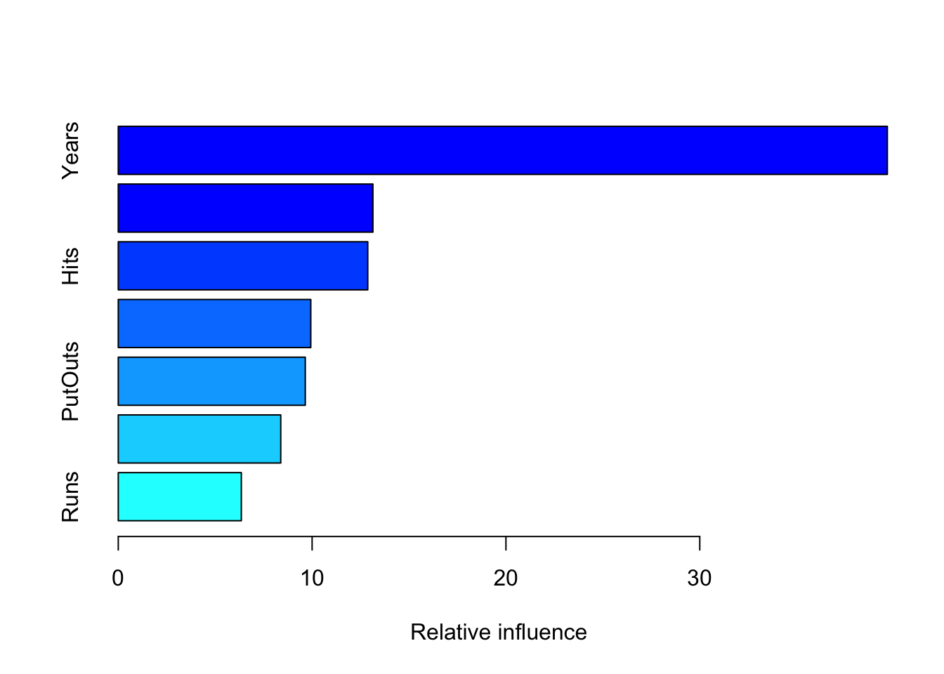
##             var   rel.inf
## Years     Years 39.678225
## Walks     Walks 13.137537
## Hits       Hits 12.871641
## RBI         RBI  9.932331
## PutOuts PutOuts  9.648024
## HmRun     HmRun  8.382579
## Runs       Runs  6.349663
We could check how the validation error changes as the number of iterations increases.
ntrees <- seq(1,1000,10)
predmat <- predict(boost.hitters, newdata=hitters2[-train,], n.trees=ntrees)
boost.err <- apply((predmat-hitters2[-train, "lgSalary"])^2, 2, mean)

plot(ntrees, boost.err, pch=19, col="darkblue", ylab="MSE", xlab="number of iterations")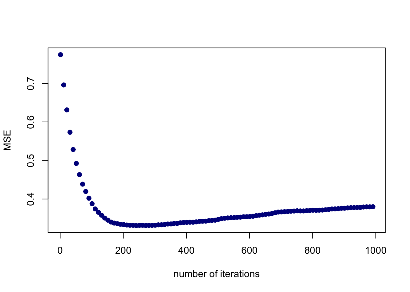
The R script for this tutorial can be found here.
This tutorial is adapted from the lab examples presented in the book “Introduction to Statistical Learning” authored by James, Witten, Hastie, & Tibshirani (2013).
© Copyright 2022 Yi Feng and Gregory R. Hancock.