EDMS 657-R Tutorial: Mixture Modeling
Yi Feng & Gregory R. Hancock
University of Maryland, College ParkIn this document we supply an example of univariate mixture modeling, an example for multivariate normal mixture, and a simple example of regression mixture using R. This document serves as a supplementary material for EDMS 657-Exploratory Latent and Composite Variable Methods, taught by Dr. Gregory R. Hancock at University of Maryland.
Before we get started, let’s install all the packages we are going to use in this demo.
install.packages("mixtools")
install.packages("FactMixtAnalysis")
install.packages("mclust")
devtools::install_github("data-edu/tidyLPA")
devtools::install_github("YiFengEDMS/EDMS657Data")
Example 1: Univariate Mixtures
Research Context
Were head circumference measurements sampled from a homogeneous normally distributed population with a single mean and variance? Were head circumference measurements sampled from a heterogeneous population consisting of multiple latent classes (i.e., unknown groups), each characterized by a normal distribution with a unique mean and variance?
Step 1: Load and examine the data
Load the data into the R session.
library(EDMS657Data)
data(ME_dat)
Take a look at the data
str(ME_dat)## 'data.frame': 2028 obs. of 4 variables:
## $ ID : chr "2000011" "2000051" "2000091" "2000101" ...
## $ sex: int 0 0 0 1 1 1 0 1 1 1 ...
## $ age: int 32 36 4 44 6 3 4 12 44 7 ...
## $ y : num 53.3 47 39 49 17 ...head(ME_dat)## ID sex age y
## 1 2000011 0 32 53.33333
## 2 2000051 0 36 47.00000
## 3 2000091 0 4 39.00000
## 4 2000101 1 44 49.00000
## 5 2000121 1 6 17.00000
## 6 2000141 1 3 34.00000Step 2: Explore the data with descriptive statistics and plots
hist(ME_dat$y, main="Child Head Circumference",
     xlab="Circumference", ylab="")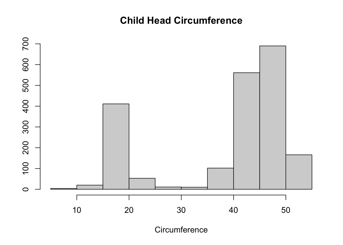
Step 3: Fit mixture models
There are many different R packages that can be used to fit mixture
models. Here I will demo this same example with three available R
packages: mixtools, mclust, and
tidyLPA.
1. mixtools package
You can use the normalmixEM function within the
mixtools R package to fit the mixture models. You will need
to specify the initial or starting values for the model parameters:
mixing proportions (lambda), means (mu), and variances (sigma).
library(mixtools)

mod1 <- normalmixEM(ME_dat$y, lambda = .5, mu = c(45, 15), sigma = c(100, 110))
## number of iterations= 28# summarize output
mod1[c("lambda", "mu", "sigma")]## $lambda
## [1] 0.7566855 0.2433145
##
## $mu
## [1] 45.65962 18.25173
##
## $sigma
## [1] 3.863324 2.380447summary(mod1)## summary of normalmixEM object:
## comp 1 comp 2
## lambda 0.756685 0.243315
## mu 45.659616 18.251726
## sigma 3.863324 2.380447
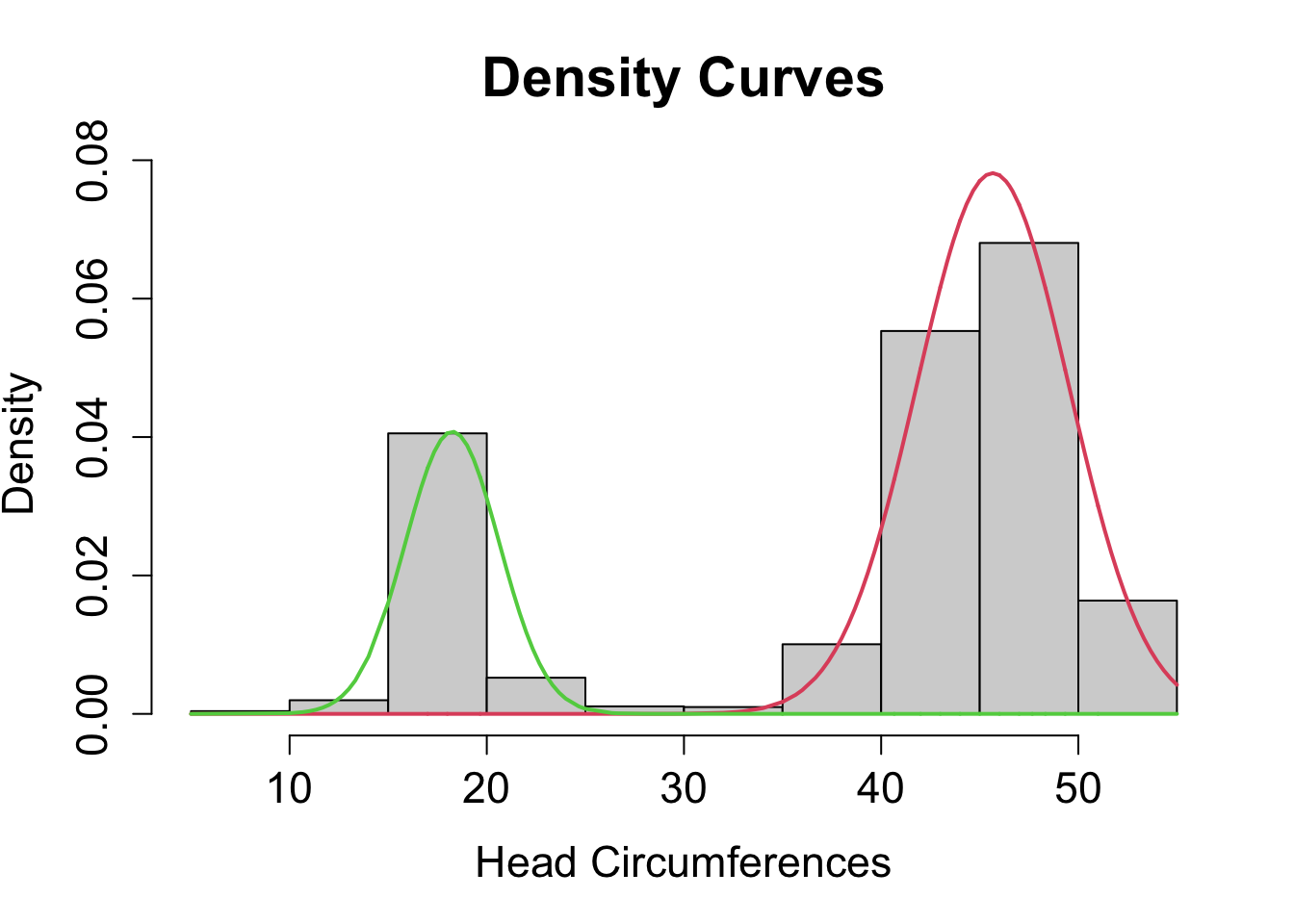
## loglik at estimate: -6501.699You could obtain a histogram of the raw data along with the two density curves determined by the model estimates.
plot(mod1, density=TRUE, cex.axis=1.4, cex.lab=1.4, cex.main=1.8, xlab2="Head Circumferences")
2. mclust package
A more commonly used R package for mixture modeling is the
mclust package. Here you do not need to supply the initial
values for the model parameters.
library(mclust)

mod4 <- densityMclust(ME_dat$y, modelName = "V", G = 2)
## fitting ...
##
|
| | 0%
|
|================================ | 50%
|
|================================================================| 100%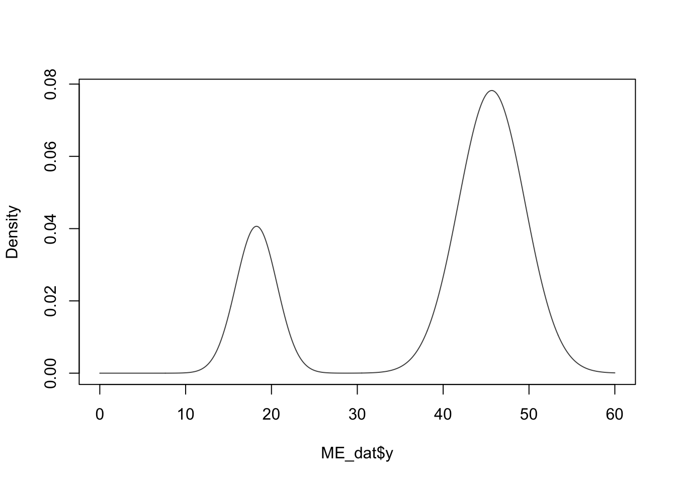
summary(mod4)## -------------------------------------------------------
## Density estimation via Gaussian finite mixture modeling
## -------------------------------------------------------
##
## Mclust V (univariate, unequal variance) model with 2 components:
##
## log-likelihood n df BIC ICL
## -6501.72 2028 5 -13041.51 -13044.59mod4$parameters## $pro
## [1] 0.2434123 0.7565877
##
## $mean
## 1 2
## 18.25592 45.66181
##
## $variance
## $variance$modelName
## [1] "V"
##
## $variance$d
## [1] 1
##
## $variance$G
## [1] 2
##
## $variance$sigmasq
## [1] 5.708087 14.889938
##
## $variance$scale
## [1] 5.708087 14.889938It is not required for you to specify the number of groups
(G =) with mclust. If you do not specify the
number of groups, mclust will run a series of models with
different numbers of groups, and determine how many clusters to keep
based on fit indices. For example:
mod5 <- densityMclust(faithful$waiting)## fitting ...
##
|
| | 0%
|
|=== | 5%
|
|======= | 11%
|
|========== | 16%
|
|============= | 21%
|
|================= | 26%
|
|==================== | 32%
|
|======================== | 37%
|
|=========================== | 42%
|
|============================== | 47%
|
|================================== | 53%
|
|===================================== | 58%
|
|======================================== | 63%
|
|============================================ | 68%
|
|=============================================== | 74%
|
|=================================================== | 79%
|
|====================================================== | 84%
|
|========================================================= | 89%
|
|============================================================= | 95%
|
|================================================================| 100%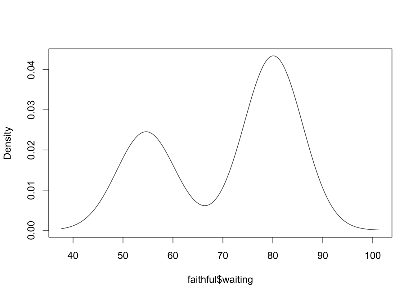
plot(mod5, what = "BIC")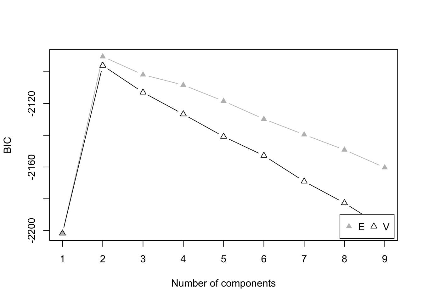
Here V represents the models that allow
varying variances across groups, while E
represents the models that contrain equal variances
across groups.
You may also note the mclust package determines the best
model by maximizing the BIC, instead of minimizing it as we have learned
in class. It is because mclust uses a slightly different
function to compute BIC compared to the general definition of it.
The general definition of BIC is: \[BIC = -2 \times ln(L(\mathbf{\Theta} | \mathbf{X})) + k \times ln(n),\] where k is the number of model parameters to be estimated.
In mclust, however, the formula for BIC is (Scrucca,
Fop, Murphy, & Raftery, 2016):
\[BIC = 2 \times ln(L(\mathbf{\Theta} |
\mathbf{X})) - k \times ln(n)\] Therefore, it makes sense that
you need to maximize BIC if using mclust.
3. tidyLPA package
You may notice that unlike Mplus, mclust does not report
entropy for the mixture models. If you need entropy, you could use the
tidyLPA R package that provides a tidy and concise wrapper
function for fitting mixture models using mclust.
library(tidyLPA)

mod6 <- estimate_profiles(ME_dat[, "y"], 1:2, variances = "varying")

mod6$model_2_class_2$estimates
## Category Parameter Estimate se p Class Model
## 1 Means df 18.255900 0.11203300 0.000000e+00 1 2
## 2 Variances df 5.707914 0.96558599 3.393213e-09 1 2
## 3 Means df 45.661800 0.09795117 0.000000e+00 2 2
## 4 Variances df 14.890084 0.67651556 2.311695e-107 2 2
## Classes
## 1 2
## 2 2
## 3 2
## 4 2Example 2: Multivariate Mixtures
data("faithful")

psych::describe(faithful)
## vars n mean sd median trimmed mad min max range skew
## eruptions 1 272 3.49 1.14 4 3.53 0.95 1.6 5.1 3.5 -0.41
## waiting 2 272 70.90 13.59 76 71.50 11.86 43.0 96.0 53.0 -0.41
## kurtosis se
## eruptions -1.51 0.07
## waiting -1.16 0.82with(faithful, plot(eruptions, waiting))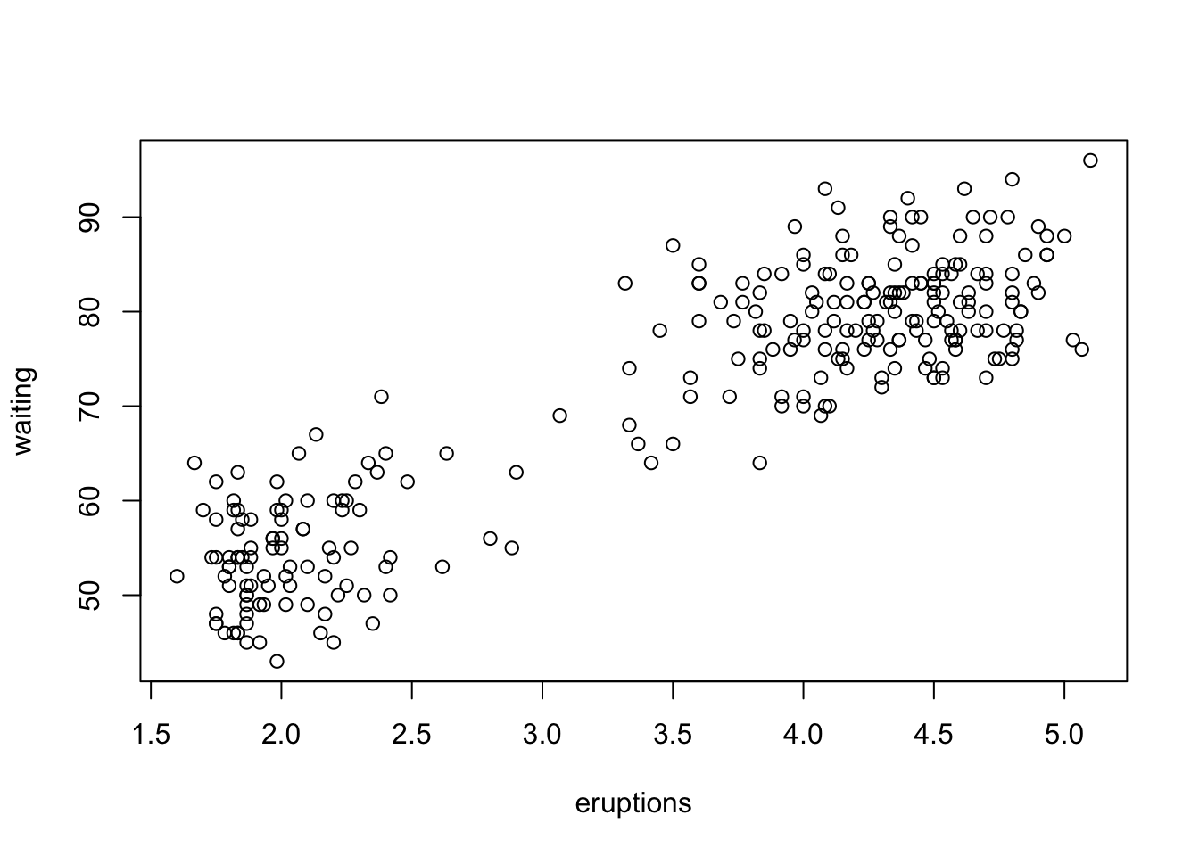
# Two clusters
out.faith <- mvnormalmixEM(faithful, arbvar = T, k = 2)
## number of iterations= 12summary(out.faith)## summary of mvnormalmixEM object:
## comp 1 comp 2
## lambda 0.355873 0.644127
## mu1 2.036389 54.478518
## mu2 4.289662 79.968117
## loglik at estimate: -1130.264out.faith$sigma## [[1]]
## [,1] [,2]
## [1,] 0.06916781 0.4351691
## [2,] 0.43516911 33.6972922
##
## [[2]]
## [,1] [,2]
## [1,] 0.1699682 0.9406068
## [2,] 0.9406068 36.0461825head(out.faith$posterior)## comp.1 comp.2
## [1,] 2.592412e-09 1.000000e+00
## [2,] 1.000000e+00 1.907899e-09
## [3,] 8.422465e-06 9.999916e-01
## [4,] 9.999893e-01 1.066832e-05
## [5,] 1.001461e-21 1.000000e+00
## [6,] 9.926681e-01 7.331888e-03plot(out.faith, which = 2)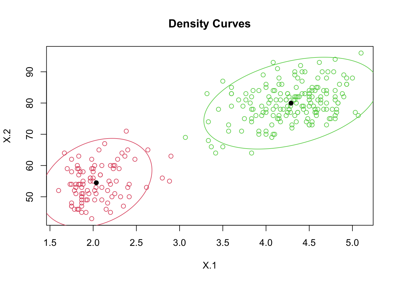
pred <- apply(out.faith$posterior, 1, function(row) which.max(row))
head(pred)
## [1] 2 1 2 1 2 1table(pred)## pred
## 1 2
## 97 175# Three clusters
out.faith3 <- mvnormalmixEM(faithful, arbvar = T, k = 3)## number of iterations= 172summary(out.faith3)## Warning in rbind(x$lambda, matrix(unlist(x$mu), byrow = TRUE, nrow =
## length(x$lambda))): number of columns of result is not a multiple of
## vector length (arg 1)## summary of mvnormalmixEM object:
## comp 1 comp 2
## lambda 0.332768 0.0903426
## mu1 1.996646 54.3829144
## mu2 3.568137 70.2600748
## mu3 4.335336 80.5227071
## loglik at estimate: -1119.214out.faith3$sigma## [[1]]
## [,1] [,2]
## [1,] 0.04390206 0.3440483
## [2,] 0.34404832 33.7411354
##
## [[2]]
## [,1] [,2]
## [1,] 0.5536093 7.849662
## [2,] 7.8496620 134.878891
##
## [[3]]
## [,1] [,2]
## [1,] 0.1359341 0.358164
## [2,] 0.3581640 28.587349head(out.faith3$posterior)## comp.1 comp.2 comp.3
## [1,] 1.139900e-13 0.125396216 8.746038e-01
## [2,] 9.984080e-01 0.001591990 7.205475e-14
## [3,] 7.855305e-09 0.593925180 4.060748e-01
## [4,] 9.903475e-01 0.009652477 3.485977e-08
## [5,] 3.293286e-33 0.051445238 9.485548e-01
## [6,] 2.276152e-03 0.997720863 2.984782e-06plot(out.faith3, which = 2)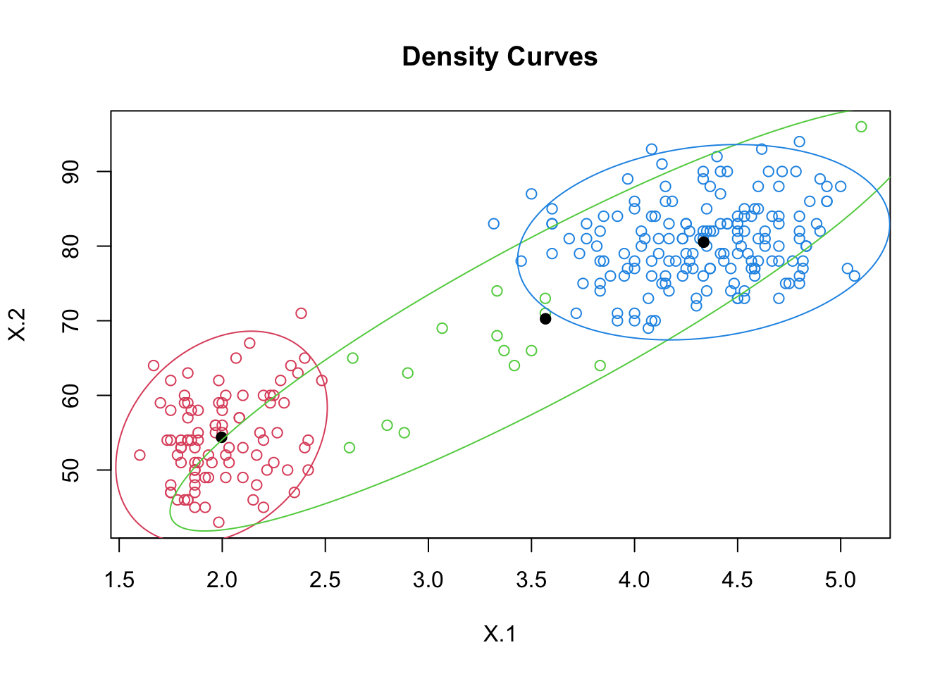
pred3 <- apply(out.faith3$posterior, 1, function(row) which.max(row))
head(pred3)
## [1] 3 1 2 1 3 2table(pred3)## pred3
## 1 2 3
## 92 15 165Example 3: Regression Mixtures
data(NOdata)

psych::describe(NOdata)
## vars n mean sd median trimmed mad min max range skew
## NO 1 88 1.96 1.13 1.75 1.91 1.44 0.37 4.03 3.66 0.33
## Equivalence 2 88 0.93 0.20 0.93 0.93 0.26 0.54 1.23 0.70 -0.14
## kurtosis se
## NO -1.30 0.12
## Equivalence -1.24 0.02with(NOdata, plot(y = Equivalence, x = NO))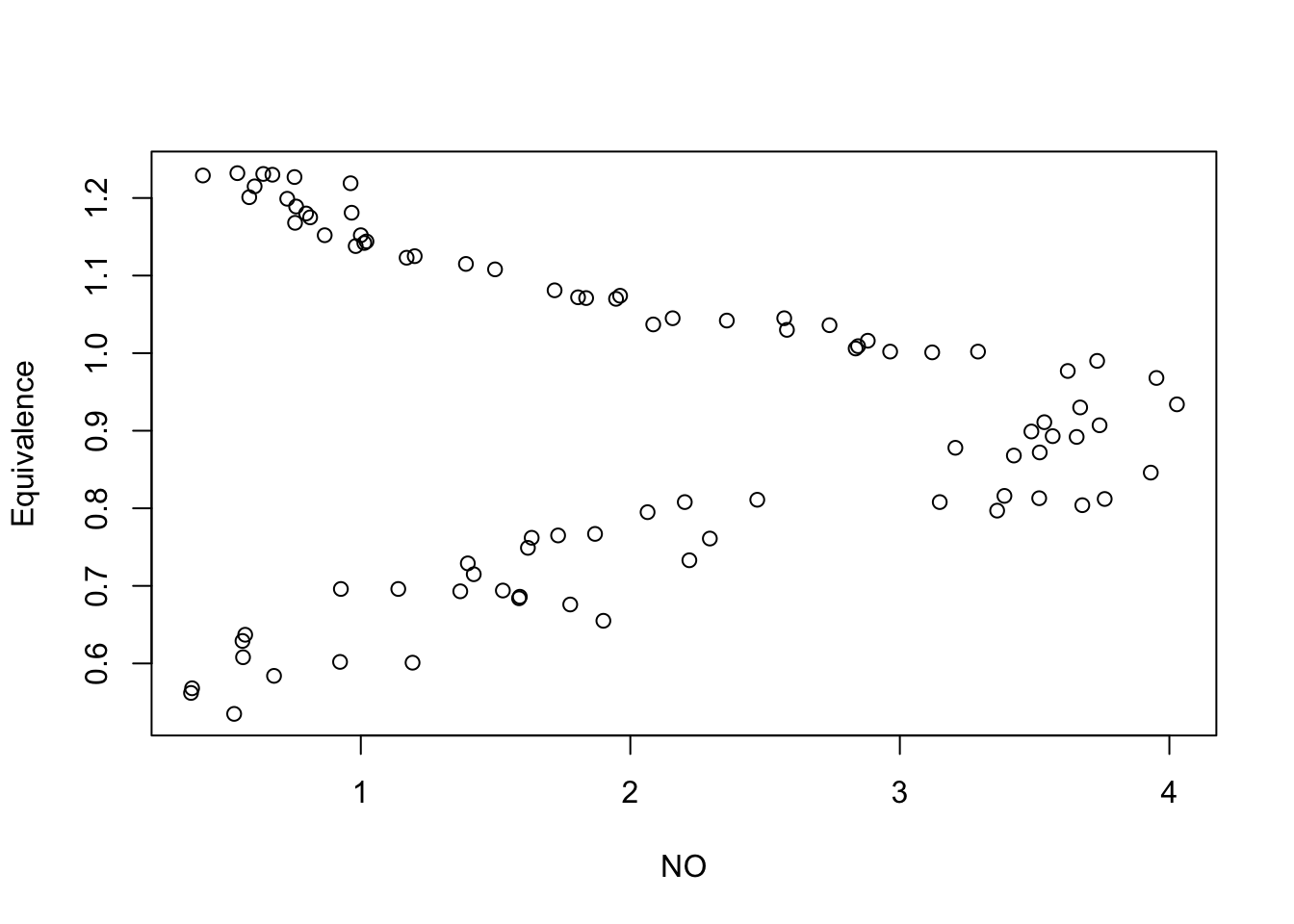
reg.out <- with(NOdata, regmixEM(y = Equivalence, x = NO, verb = F, epsilon = 1e-04, k = 2))## number of iterations= 18summary(reg.out)## summary of regmixEM object:
## comp 1 comp 2
## lambda 0.4897277 0.5102723
## sigma 0.0433292 0.0241435
## beta1 0.5649610 1.2471261
## beta2 0.0850408 -0.0830369
## loglik at estimate: 122.0383reg.out[3:6]## $lambda
## [1] 0.4897277 0.5102723
##
## $beta
## comp.1 comp.2
## beta.0 0.56496100 1.24712608
## beta.1 0.08504084 -0.08303687
##
## $sigma
## [1] 0.04332924 0.02414351
##
## $loglik
## [1] 122.0383plot(reg.out, which = 2, xlab2 = "NO", ylab2 = "Equivalence")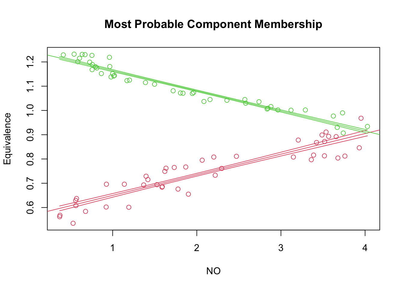
The R script for this tutorial can be found here.
References
Scrucca, L., Fop, M., Murphy, T. B., & Raftery, A. E. (2016). mclust 5: clustering, classification and density estimation using Gaussian finite mixture models. The R Journal, 8, 289-317.
© Copyright 2022 Yi Feng and Gregory R. Hancock.