EDMS 657-R Tutorial: MANOVA

In this document we supply three simple examples of MANOVA using R. This document serves as a supplementary material for EDMS 657-Exploratory Latent and Composite Variable Methods, taught by Dr. Gregory R. Hancock at University of Maryland.

Before we get started, let’s install all the packages we are going to use in this demo.

install.packages("tidyverse")
install.packages("ggplot2")
install.packages("gridExtra")
install.packages("heplots")
install.packages("agricolae")
install.packages("candisc")
install.packages("MASS")
install.packages("Hmisc")
devtools::install_github("YiFengEDMS/EDMS657Data")

Example 1: Two-group MANOVA / Hoteling’s \(T^2\)

Research Context

Middle school students are randomly assigned to an educational treatment or a control group. After receiving their treatment or control experience, students are evaluated in terms of cognitive and affective outcomes together. We are interested in testing whether there is any difference between the treatment/control groups regarding the set of outcomes.

Step 1: Read and examine the data

Load the data into the R session.

library(EDMS657Data)
data(Hotellings_T)

Take a look at the data

library(tidyverse)
#View(Hotellings_T)
glimpse(Hotellings_T)

## Rows: 30
## Columns: 3
## $ treat    <dbl> 1, 1, 1, 1, 1, 1, 1, 1, 1, 1, 1, 1, 1, 1, 1, 2, 2, 2, 2…
## $ attitude <dbl> 4, 5, 6, 6, 7, 8, 8, 9, 10, 10, 11, 11, 12, 12, 13, 8, …
## $ know     <dbl> 14, 14, 16, 20, 17, 15, 18, 13, 15, 21, 11, 12, 15, 24,…

str(Hotellings_T)

## 'data.frame':    30 obs. of  3 variables:
##  $ treat   : num  1 1 1 1 1 1 1 1 1 1 ...
##   ..- attr(*, "value.labels")= Named chr [1:2] "2" "1"
##   .. ..- attr(*, "names")= chr [1:2] "control" "experimental"
##  $ attitude: num  4 5 6 6 7 8 8 9 10 10 ...
##  $ know    : num  14 14 16 20 17 15 18 13 15 21 ...
##  - attr(*, "variable.labels")= Named chr [1:3] "treatment condition" "attitude toward people with HIV/AIDS" "HIV/AIDS knowledge test"
##   ..- attr(*, "names")= chr [1:3] "treat" "attitude" "know"
##  - attr(*, "codepage")= int 65001

head(Hotellings_T)

##   treat attitude know
## 1     1        4   14
## 2     1        5   14
## 3     1        6   16
## 4     1        6   20
## 5     1        7   17
## 6     1        8   15

Note that “treatment” should be a categorical variable.

Hotellings_T <- Hotellings_T %>% 
  mutate(treat = factor(treat, labels = c("experimental", "control")))

Step 2: Explore the data with descriptive statistics and plots

Descriptive statistics

summary(Hotellings_T)

##           treat       attitude          know      
##  experimental:15   Min.   : 4.00   Min.   :10.00  
##  control     :15   1st Qu.: 8.25   1st Qu.:13.25  
##                    Median :11.50   Median :15.00  
##                    Mean   :11.47   Mean   :15.43  
##                    3rd Qu.:14.00   3rd Qu.:17.00  
##                    Max.   :19.00   Max.   :24.00

table(Hotellings_T$treat)

## 
## experimental      control 
##           15           15

You can get the within-group means:

Hotellings_T %>% 
  group_by(treat) %>% 
  summarize(mean_att = mean(attitude),
            mean_know = mean(know))

## # A tibble: 2 × 3
##   treat        mean_att mean_know
##   <fct>           <dbl>     <dbl>
## 1 experimental      8.8      16.2
## 2 control          14.1      14.7

You can get the within-group variances:

Hotellings_T %>% 
  group_by(treat) %>% 
  summarize(var_att = var(attitude),
            var_know = var(know))

## # A tibble: 2 × 3
##   treat        var_att var_know
##   <fct>          <dbl>    <dbl>
## 1 experimental    7.74    12.5 
## 2 control        10.4      6.95

Or alternatively, examine group statistics altogether:

psych::describeBy(attitude + know ~ treat, data = Hotellings_T)

## 
##  Descriptive statistics by group 
## treat: experimental
##          vars  n mean   sd median trimmed  mad min max range  skew
## attitude    1 15  8.8 2.78      9    8.85 2.97   4  13     9 -0.16
## know        2 15 16.2 3.53     15   16.00 2.97  11  24    13  0.57
##          kurtosis   se
## attitude    -1.39 0.72
## know        -0.57 0.91
## ------------------------------------------------------- 
## treat: control
##          vars  n  mean   sd median trimmed  mad min max range  skew
## attitude    1 15 14.13 3.23     14   14.23 2.97   8  19    11 -0.31
## know        2 15 14.67 2.64     15   14.62 2.97  10  20    10  0.05
##          kurtosis   se
## attitude    -0.99 0.83
## know        -0.76 0.68

Descriptive plots

Scatterplot

library(ggplot2)

# The plot is colored by the group
scatterPlot <- ggplot(Hotellings_T, aes(attitude, know, color = treat)) + 
  geom_point() + 
  scale_color_manual(values = c('#999999','#E69F00')) + 
  labs(color = "treatment condition") +
  theme_bw() +
  theme(legend.position = "bottom")
scatterPlot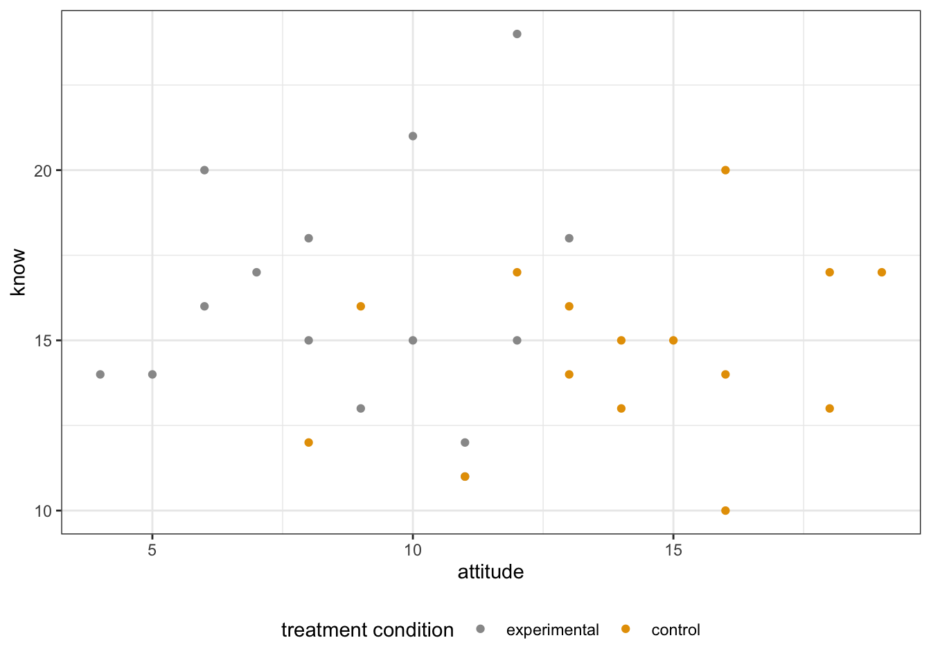

Marginal density plot of attitude

xdensity <- ggplot(Hotellings_T, aes(attitude, fill=treat)) + 
  geom_density(alpha=.5) + 
  scale_fill_manual(values = c('#999999','#E69F00')) + 
  theme(legend.position = "none")
xdensity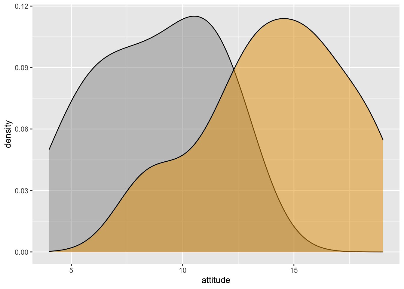

Marginal density plot of knowledge

ydensity <- ggplot(Hotellings_T, aes(know, fill=treat)) + 
  geom_density(alpha=.5) + 
  scale_fill_manual(values = c('#999999','#E69F00')) + 
  theme(legend.position = "none")
ydensity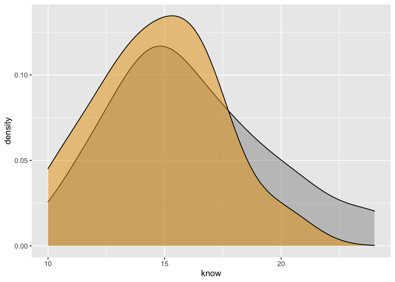

Put them all together in one plot

blankPlot <- ggplot()+geom_blank(aes(1,1))+
  theme(plot.background = element_blank(), 
        panel.grid.major = element_blank(),
        panel.grid.minor = element_blank(), 
        panel.border = element_blank(),
        panel.background = element_blank(),
        axis.title.x = element_blank(),
        axis.title.y = element_blank(),
        axis.text.x = element_blank(), 
        axis.text.y = element_blank(),
        axis.ticks = element_blank()
  )

library("gridExtra")
grid.arrange(xdensity, blankPlot, scatterPlot, ydensity, 
             ncol=2, nrow=2, widths=c(4, 1.4), heights=c(1.4, 4))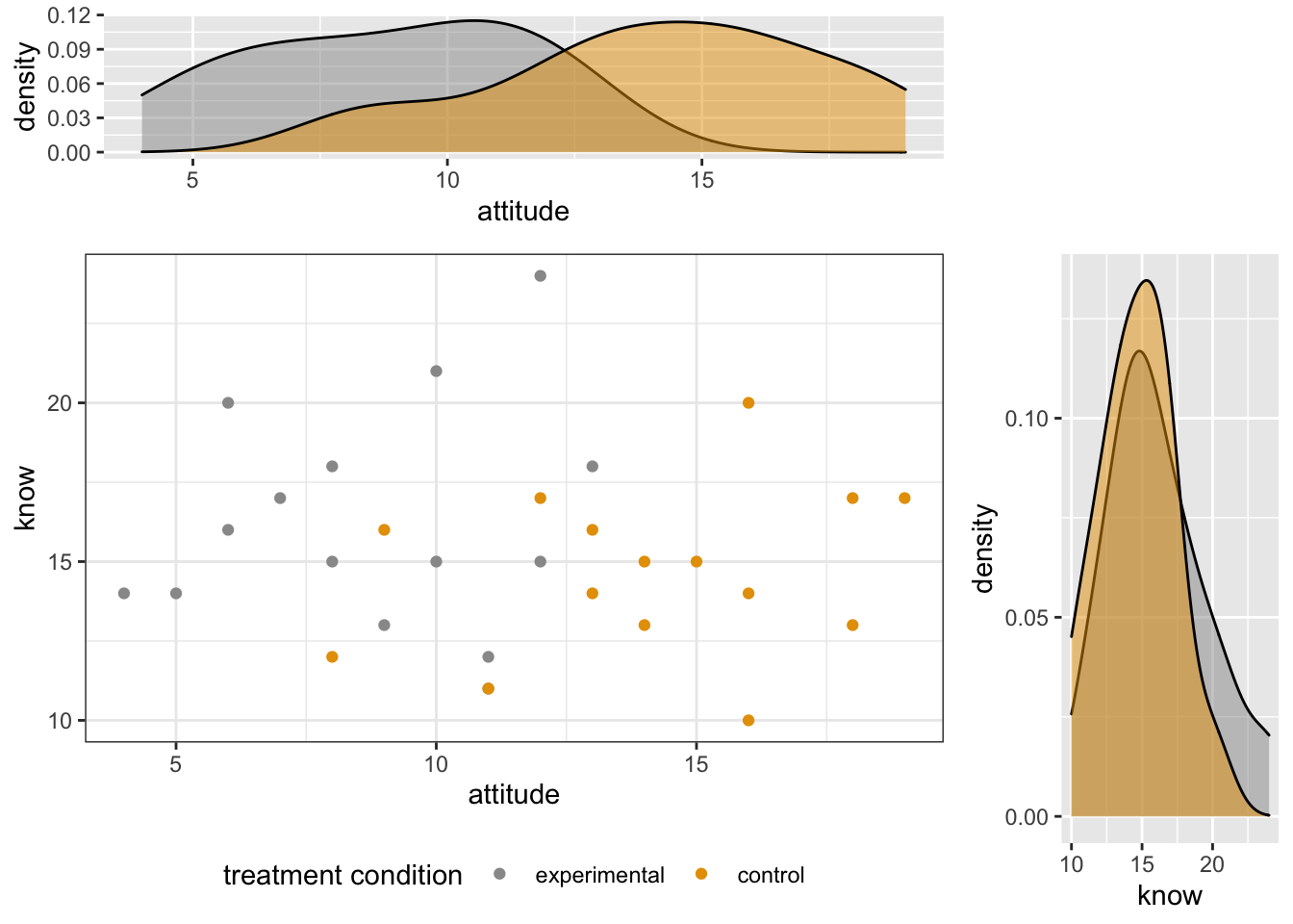

You can also add centroids to the scatterplot:

centroids <- aggregate(cbind(attitude = attitude, know = know) ~ treat, data = Hotellings_T, mean)
scatterPlot + geom_point(centroids, mapping = aes(x = attitude, y = know), size = 5, shape = 17) +  
  labs(color = "treatment condition centroids")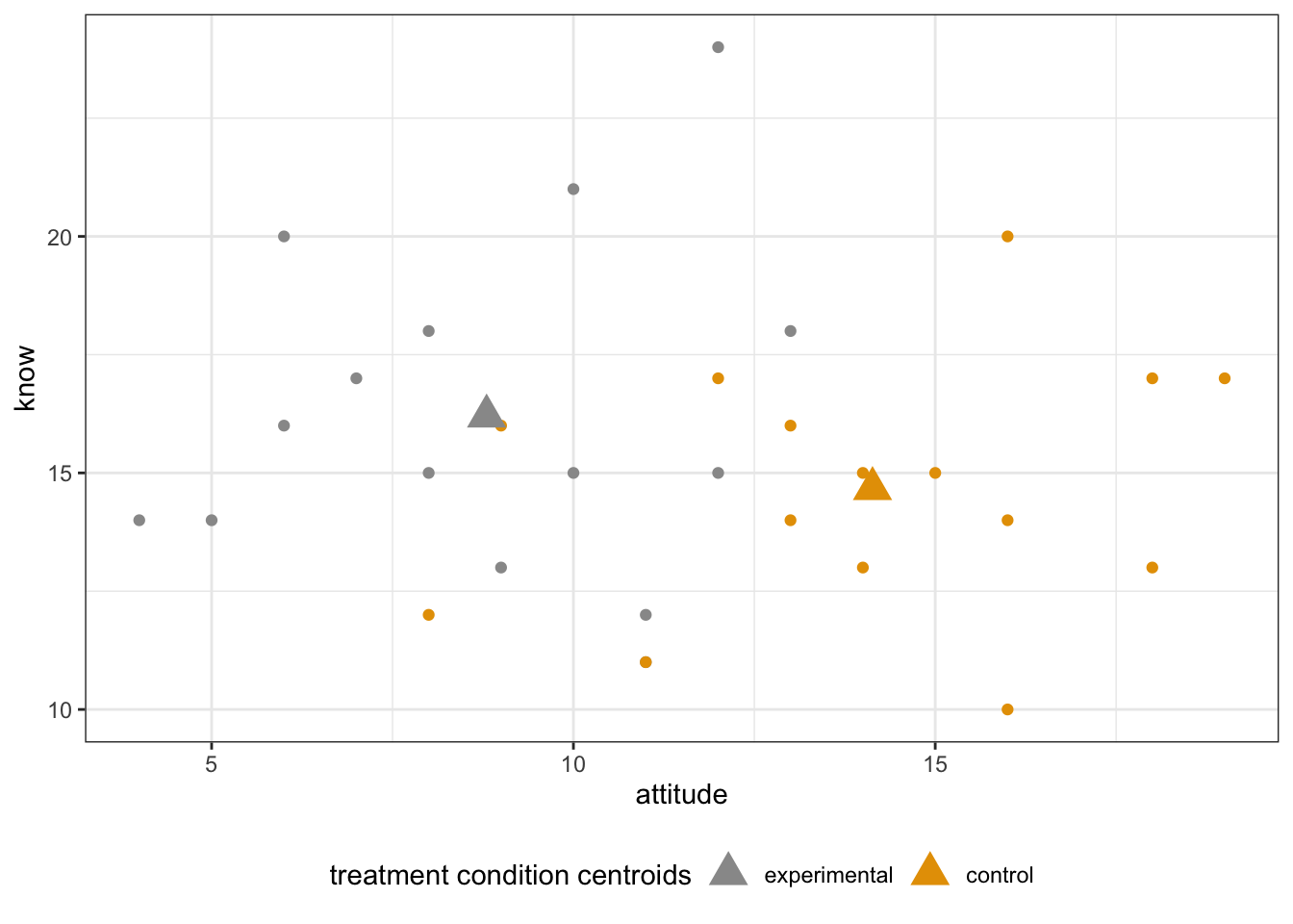

You can also do boxplots in addition to density plots.

par(mfrow = c(2, 1), mar=c(1,1,1,1))
ggplot(Hotellings_T, aes(x=treat, y=attitude, color=treat)) +
  geom_boxplot()+ theme(legend.position = "none") + 
  xlab("Treatment Condition")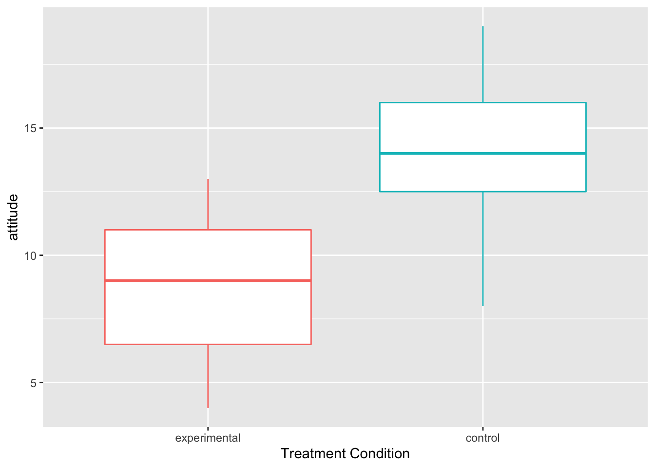

ggplot(Hotellings_T, aes(x=treat, y=know, color=treat)) +
  geom_boxplot()+ theme(legend.position = "none") + 
  xlab("Treatment Condition")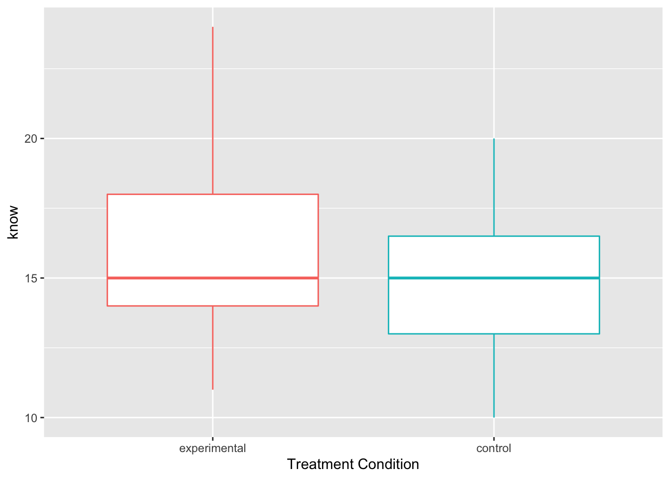

Step 3: Implement MANOVA analysis

Multivariate tests

You can obtain different types of statistics by specifying the test= argument accordingly. The default will give you Pillai’s trace.

manova.model1 <- manova(cbind(attitude = attitude, know = know) ~ treat, Hotellings_T)
summary(manova.model1, test = "Pillai", intercept=T)

##             Df  Pillai approx F num Df den Df    Pr(>F)    
## (Intercept)  1 0.97268   480.57      2     27 < 2.2e-16 ***
## treat        1 0.50609    13.83      2     27 7.316e-05 ***
## Residuals   28                                             
## ---
## Signif. codes:  0 '***' 0.001 '**' 0.01 '*' 0.05 '.' 0.1 ' ' 1

summary(manova.model1, test = "Wilks", intercept=T)

##             Df   Wilks approx F num Df den Df    Pr(>F)    
## (Intercept)  1 0.02732   480.57      2     27 < 2.2e-16 ***
## treat        1 0.49391    13.83      2     27 7.316e-05 ***
## Residuals   28                                             
## ---
## Signif. codes:  0 '***' 0.001 '**' 0.01 '*' 0.05 '.' 0.1 ' ' 1

summary(manova.model1, test = "Hotelling-Lawley", intercept=T)

##             Df Hotelling-Lawley approx F num Df den Df    Pr(>F)    
## (Intercept)  1           35.597   480.57      2     27 < 2.2e-16 ***
## treat        1            1.025    13.83      2     27 7.316e-05 ***
## Residuals   28                                                      
## ---
## Signif. codes:  0 '***' 0.001 '**' 0.01 '*' 0.05 '.' 0.1 ' ' 1

summary(manova.model1, test = "Roy", intercept=T)

##             Df    Roy approx F num Df den Df    Pr(>F)    
## (Intercept)  1 35.597   480.57      2     27 < 2.2e-16 ***
## treat        1  1.025    13.83      2     27 7.316e-05 ***
## Residuals   28                                            
## ---
## Signif. codes:  0 '***' 0.001 '**' 0.01 '*' 0.05 '.' 0.1 ' ' 1

Conduct the Box’s M test (homogeneity of dispersion)

library(heplots)

boxtest2 <- boxM(Hotellings_T[, c("attitude", "know")], Hotellings_T$treat)
summary(boxtest2)

## Summary for Box's M-test of Equality of Covariance Matrices
## 
## Chi-Sq:   1.544326 
## df:   3 
## p-value: 0.6721 
## 
## log of Covariance determinants:
## experimental      control       pooled 
##     4.550595     4.217750     4.443953 
## 
## Eigenvalues:
##   experimental control    pooled
## 1    12.805776 11.4156 11.142702
## 2     7.394224  5.9463  7.638251
## 
## Statistics based on eigenvalues:
##           experimental   control    pooled
## product      94.688776 67.880612 85.110748
## sum          20.200000 17.361905 18.780952
## precision     4.687563  3.909745  4.531759
## max          12.805776 11.415604 11.142702

Step 4: Follow-up: Univariate ANOVA

anova(lm(attitude~treat, Hotellings_T))

## Analysis of Variance Table
## 
## Response: attitude
##           Df Sum Sq Mean Sq F value    Pr(>F)    
## treat      1 213.33 213.333  23.505 4.201e-05 ***
## Residuals 28 254.13   9.076                      
## ---
## Signif. codes:  0 '***' 0.001 '**' 0.01 '*' 0.05 '.' 0.1 ' ' 1

anova(lm(know~treat, Hotellings_T))

## Analysis of Variance Table
## 
## Response: know
##           Df  Sum Sq Mean Sq F value Pr(>F)
## treat      1  17.633 17.6333   1.817 0.1885
## Residuals 28 271.733  9.7048

Example 2: Three-group MANOVA

Research Context

Middle school students are randomly assigned to one of three treatment groups. After receiving their respective treatment or control experience, students are evaluated in terms of cognitive and affective outcomes together. We are interested in testing whether there is any difference between the three treatment groups regarding the set of outcomes.

Step 1: Load the data

library(EDMS657Data)
data("manova_dat")

take a look at the data you just read into R

#View(manova.data2)
glimpse(manova_dat)

## Rows: 45
## Columns: 3
## $ treat    <dbl> 1, 1, 1, 1, 1, 1, 1, 1, 1, 1, 1, 1, 1, 1, 1, 2, 2, 2, 2…
## $ attitude <dbl> 4, 5, 6, 6, 7, 8, 8, 9, 10, 10, 11, 11, 12, 12, 13, 8, …
## $ know     <dbl> 14, 14, 16, 20, 17, 15, 18, 13, 15, 21, 11, 12, 15, 24,…

str(manova_dat)

## 'data.frame':    45 obs. of  3 variables:
##  $ treat   : num  1 1 1 1 1 1 1 1 1 1 ...
##   ..- attr(*, "value.labels")= Named chr [1:3] "3" "2" "1"
##   .. ..- attr(*, "names")= chr [1:3] "webinar" "control" "experimental"
##  $ attitude: num  4 5 6 6 7 8 8 9 10 10 ...
##  $ know    : num  14 14 16 20 17 15 18 13 15 21 ...
##  - attr(*, "variable.labels")= Named chr [1:3] "treatment condition" "attitude toward people with HIV/AIDS" "HIV/AIDS knowledge test"
##   ..- attr(*, "names")= chr [1:3] "treat" "attitude" "know"
##  - attr(*, "codepage")= int 65001

head(manova_dat)

##   treat attitude know
## 1     1        4   14
## 2     1        5   14
## 3     1        6   16
## 4     1        6   20
## 5     1        7   17
## 6     1        8   15

Again, “treatment” is a categorical variable

manova_dat$treat <- as.factor(manova_dat$treat)
levels(manova_dat$treat) <- c("experimental", "control", "webinar")

Step 2: Explore the data with descriptive statistics and plots

Descriptive statistics

summary(manova_dat)

##           treat       attitude           know      
##  experimental:15   Min.   : 4.000   Min.   : 8.00  
##  control     :15   1st Qu.: 7.000   1st Qu.:11.00  
##  webinar     :15   Median : 9.000   Median :14.00  
##                    Mean   : 9.933   Mean   :14.02  
##                    3rd Qu.:13.000   3rd Qu.:16.00  
##                    Max.   :19.000   Max.   :24.00

table(manova_dat$treat)

## 
## experimental      control      webinar 
##           15           15           15

Within-group means

with(manova_dat, tapply(attitude, treat, mean))

## experimental      control      webinar 
##     8.800000    14.133333     6.866667

with(manova_dat, tapply(know, treat, mean))

## experimental      control      webinar 
##     16.20000     14.66667     11.20000

Within-group variances

with(manova_dat, tapply(attitude, treat, var))

## experimental      control      webinar 
##     7.742857    10.409524     4.552381

with(manova_dat, tapply(know, treat, var))

## experimental      control      webinar 
##    12.457143     6.952381     3.314286

psych::describeBy(attitude + know ~ treat, data = manova_dat)

## 
##  Descriptive statistics by group 
## treat: experimental
##          vars  n mean   sd median trimmed  mad min max range  skew
## attitude    1 15  8.8 2.78      9    8.85 2.97   4  13     9 -0.16
## know        2 15 16.2 3.53     15   16.00 2.97  11  24    13  0.57
##          kurtosis   se
## attitude    -1.39 0.72
## know        -0.57 0.91
## ------------------------------------------------------- 
## treat: control
##          vars  n  mean   sd median trimmed  mad min max range  skew
## attitude    1 15 14.13 3.23     14   14.23 2.97   8  19    11 -0.31
## know        2 15 14.67 2.64     15   14.62 2.97  10  20    10  0.05
##          kurtosis   se
## attitude    -0.99 0.83
## know        -0.76 0.68
## ------------------------------------------------------- 
## treat: webinar
##          vars  n  mean   sd median trimmed  mad min max range  skew
## attitude    1 15  6.87 2.13      7    6.77 2.97   4  11     7  0.33
## know        2 15 11.20 1.82     11   11.23 1.48   8  14     6 -0.01
##          kurtosis   se
## attitude    -1.11 0.55
## know        -1.18 0.47

Descriptive plots

Scatterplot

library(ggplot2)

scatterPlot2 <- ggplot(manova_dat, aes(attitude, know, color=treat)) + 
  geom_point() + 
  scale_color_manual(values = c("#999999", "#E69F00", "#56B4E9")) + 
  labs(color="treatment condition") +
  theme_bw() +
  theme(legend.position = "bottom")
scatterPlot2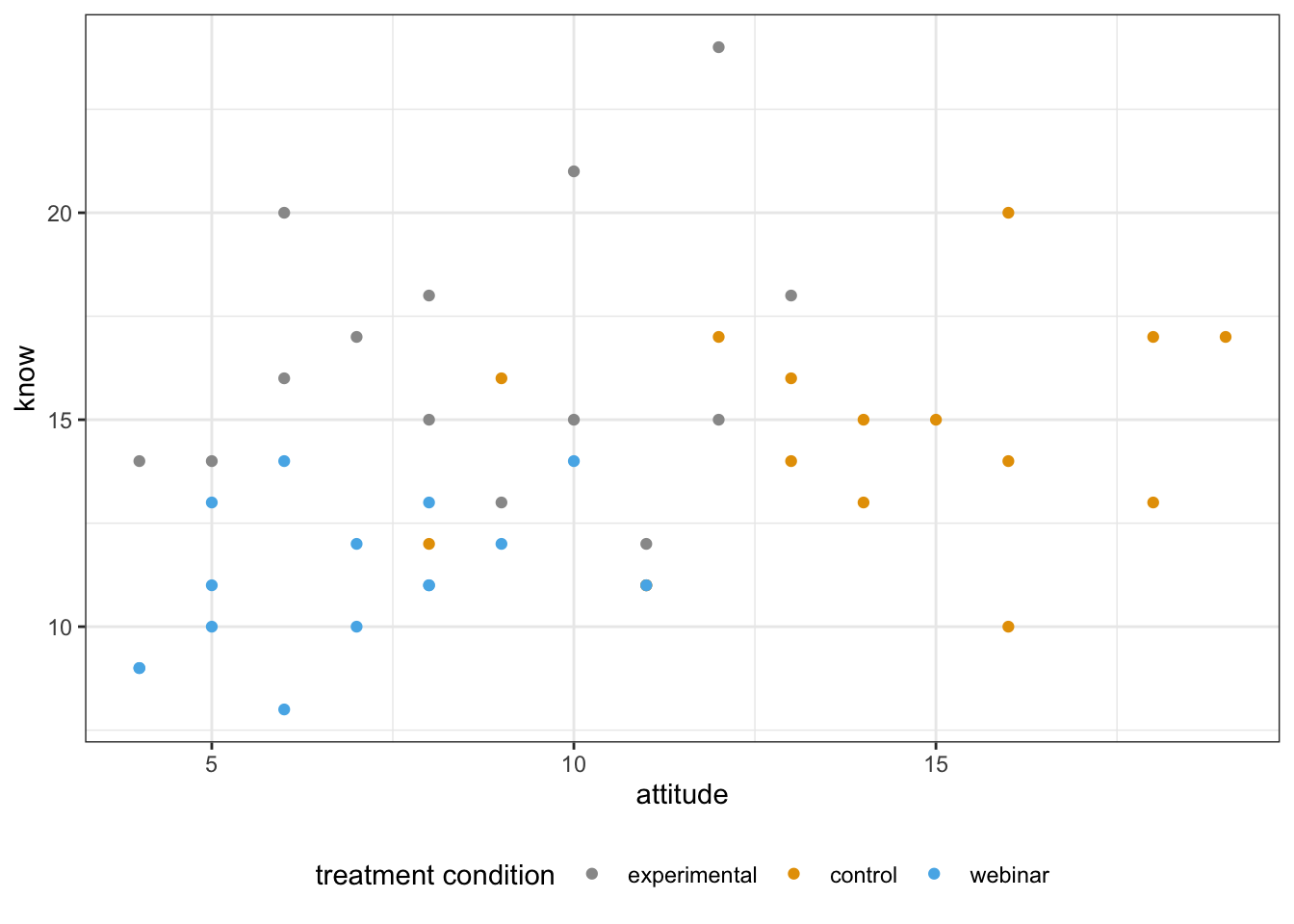

xdensity2 <- ggplot(manova_dat, aes(attitude, fill=treat)) + 
  geom_density(alpha=.5) + 
  scale_fill_manual(values = c("#999999", "#E69F00", "#56B4E9")) + 
  theme(legend.position = "none")
xdensity2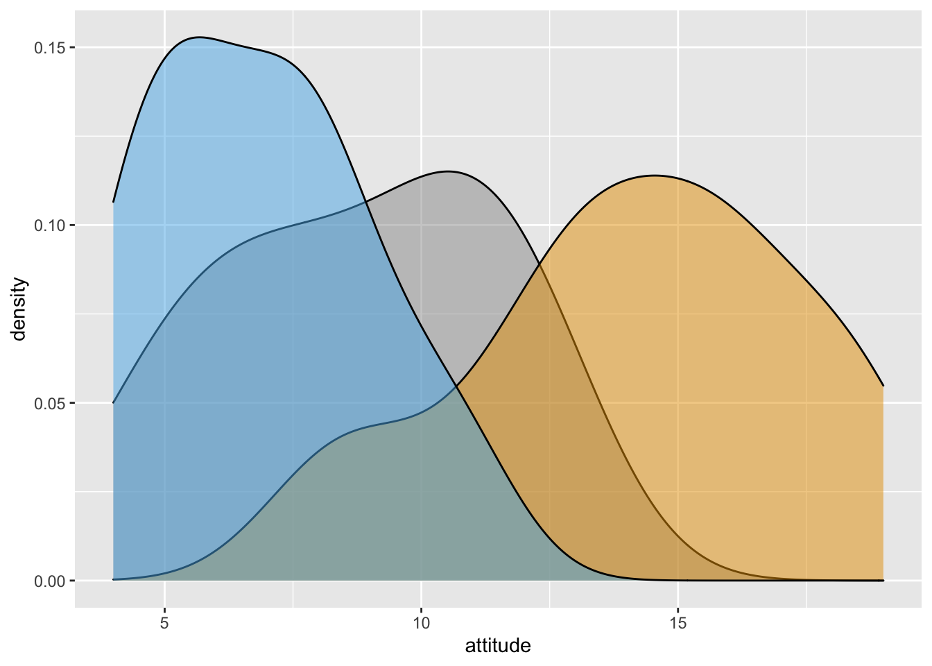

ydensity2 <- ggplot(manova_dat, aes(know, fill=treat)) + 
  geom_density(alpha=.5) + 
  scale_fill_manual(values = c("#999999", "#E69F00", "#56B4E9")) + 
  theme(legend.position = "none")
ydensity2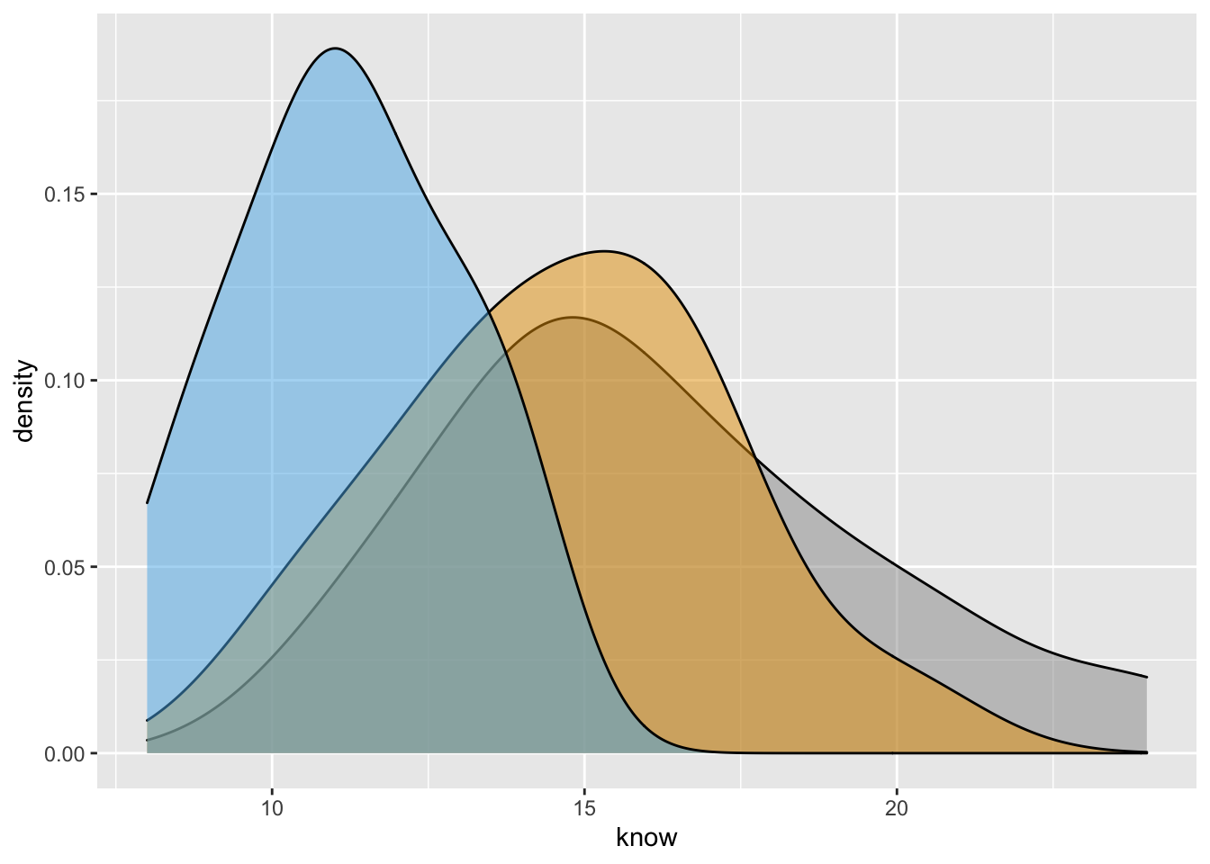

blankPlot <- ggplot()+geom_blank(aes(1,1))+
  theme(plot.background = element_blank(), 
        panel.grid.major = element_blank(),
        panel.grid.minor = element_blank(), 
        panel.border = element_blank(),
        panel.background = element_blank(),
        axis.title.x = element_blank(),
        axis.title.y = element_blank(),
        axis.text.x = element_blank(), 
        axis.text.y = element_blank(),
        axis.ticks = element_blank()
  )

library("gridExtra")
grid.arrange(xdensity2, blankPlot, scatterPlot2, ydensity2, 
             ncol=2, nrow=2, widths=c(4, 1.4), heights=c(1.4, 4))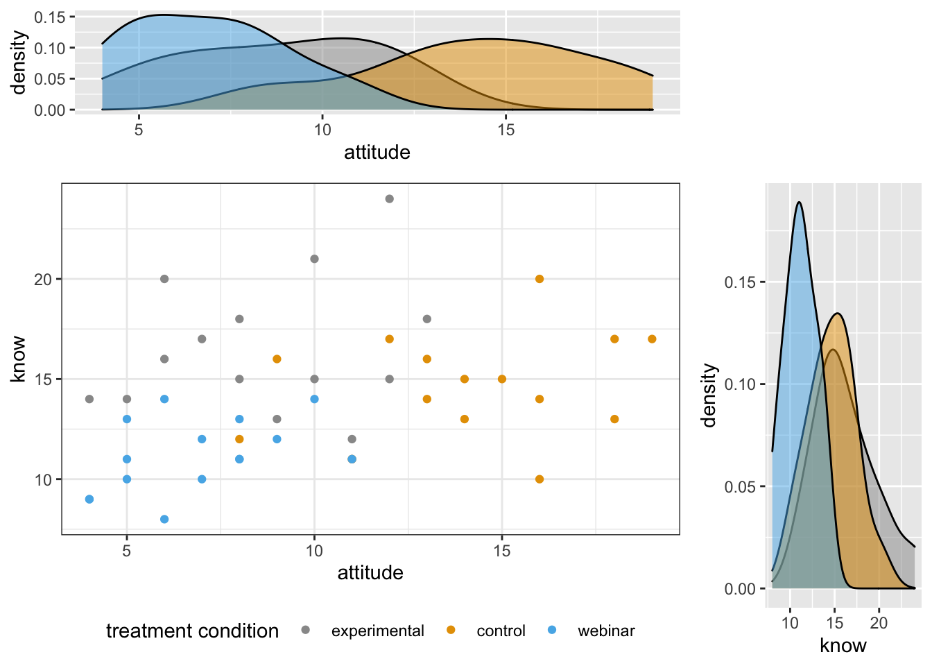

Add centroids

centroids2 <- aggregate(cbind(attitude = attitude, know = know)~treat, data = manova_dat, mean)
scatterPlot2 + geom_point(centroids2,mapping=aes(x=attitude,y=know),size=5,shape=17)+  
  labs(color="treatment condition centroids")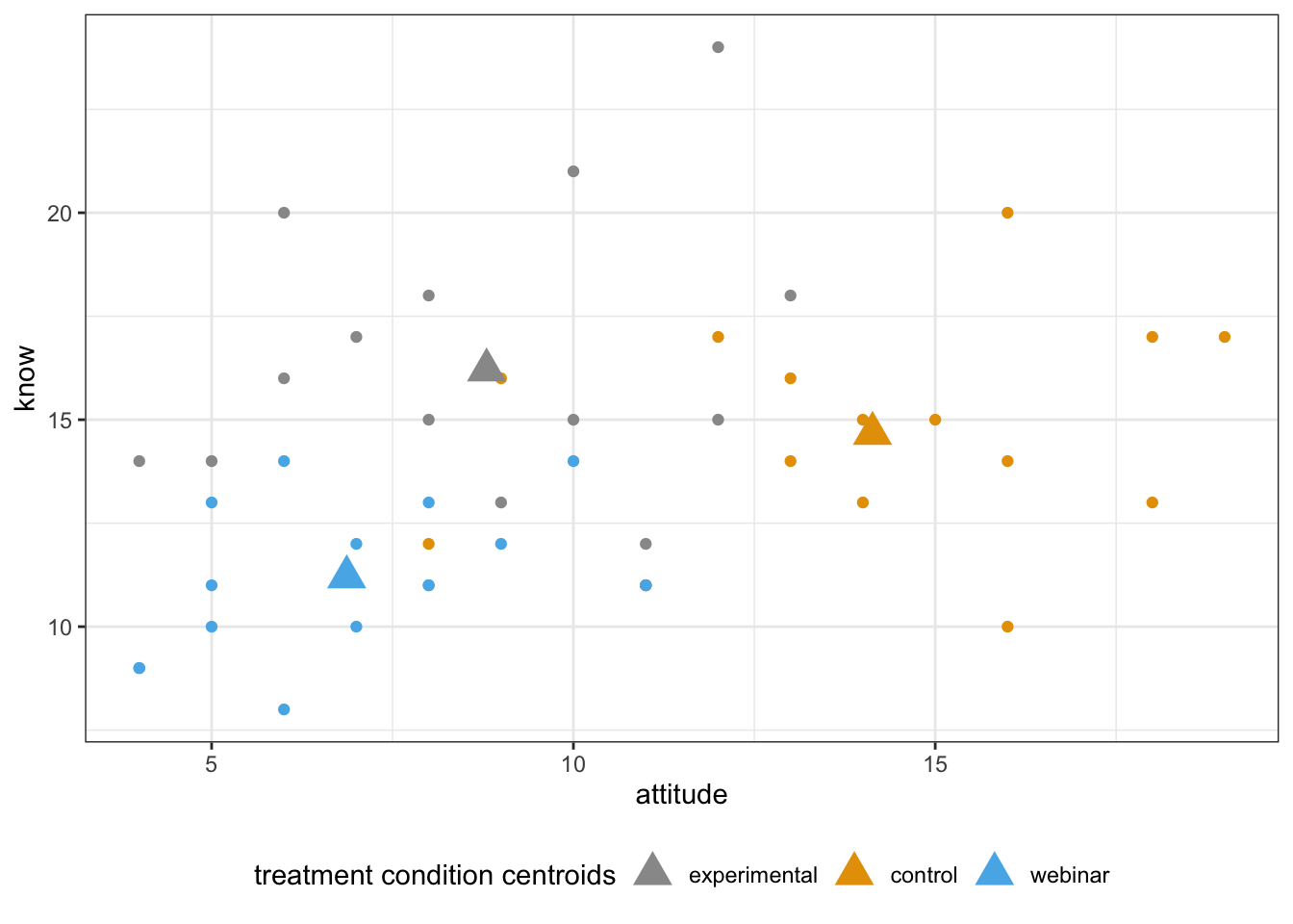

Boxplots

ggplot(manova_dat, aes(x=treat, y=attitude, color=treat)) +
  geom_boxplot()+ theme(legend.position = "none") + 
  xlab("Treatment Condition")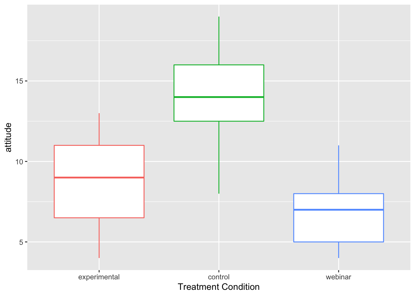

ggplot(manova_dat, aes(x=treat, y=know, color=treat)) +
  geom_boxplot()+ theme(legend.position = "none") + 
  xlab("Treatment Condition")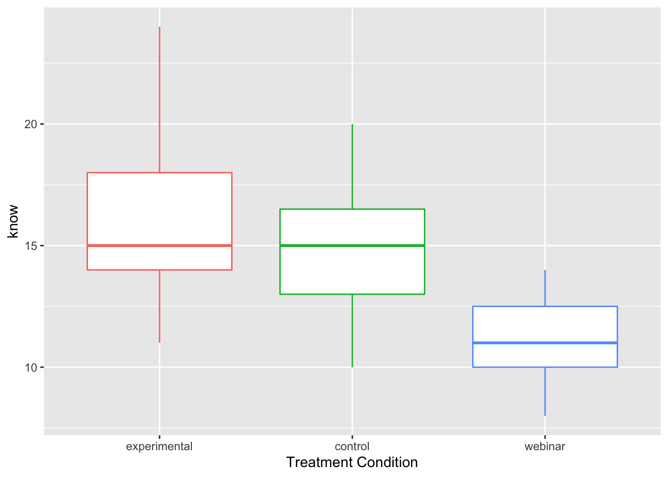

Raincloud plots

Inspired by this online post by Dr. Allen, we could do raincloud plots to describe the data.

source("https://gist.githubusercontent.com/benmarwick/2a1bb0133ff568cbe28d/raw/fb53bd97121f7f9ce947837ef1a4c65a73bffb3f/geom_flat_violin.R")


raincloud_theme = theme(
text = element_text(size = 10),
axis.title.x = element_text(size = 16),
axis.title.y = element_text(size = 16),
axis.text = element_text(size = 14),
axis.text.x = element_text(angle = 45, vjust = 0.5),
legend.title=element_text(size=16),
legend.text=element_text(size=16),
legend.position = "right",
plot.title = element_text(lineheight=.8, face="bold", size = 16),
panel.border = element_blank(),
panel.grid.minor = element_blank(),
panel.grid.major = element_blank(),
axis.line.x = element_line(colour = 'black', size=0.5, linetype='solid'),
axis.line.y = element_line(colour = 'black', size=0.5, linetype='solid'))

rc_plot <- ggplot(data = manova_dat, aes(x=treat, y=attitude, fill = treat)) +
geom_flat_violin(position = position_nudge(x = .2, y = 0), alpha = .8) +
geom_point(aes(y=attitude, color = treat), position = position_jitter(width = .15), size = .5, alpha = 0.8) +
geom_boxplot(width = .1, guides = FALSE, outlier.shape = NA, alpha = 0.5) +
expand_limits(x = 4, y = 20) +
guides(fill = FALSE) +
guides(color = FALSE) +
scale_color_brewer(palette = "Set1") +
scale_fill_brewer(palette = "Set1") +
theme_bw() +
raincloud_theme

rc_plot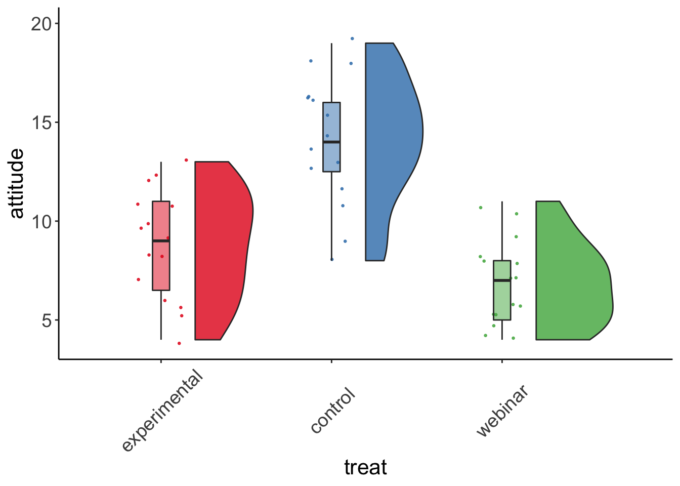

rc_plot2 <- ggplot(data = manova_dat, aes(x=treat, y=know, fill = treat)) +
geom_flat_violin(position = position_nudge(x = .2, y = 0), alpha = .8) +
geom_point(aes(y=know, color = treat), position = position_jitter(width = .15), size = .5, alpha = 0.8) +
geom_boxplot(width = .1, guides = FALSE, outlier.shape = NA, alpha = 0.5) +
expand_limits(x = 4, y = 20) +
guides(fill = FALSE) +
guides(color = FALSE) +
scale_color_brewer(palette = "Set1") +
scale_fill_brewer(palette = "Set1") +
theme_bw() +
raincloud_theme

rc_plot2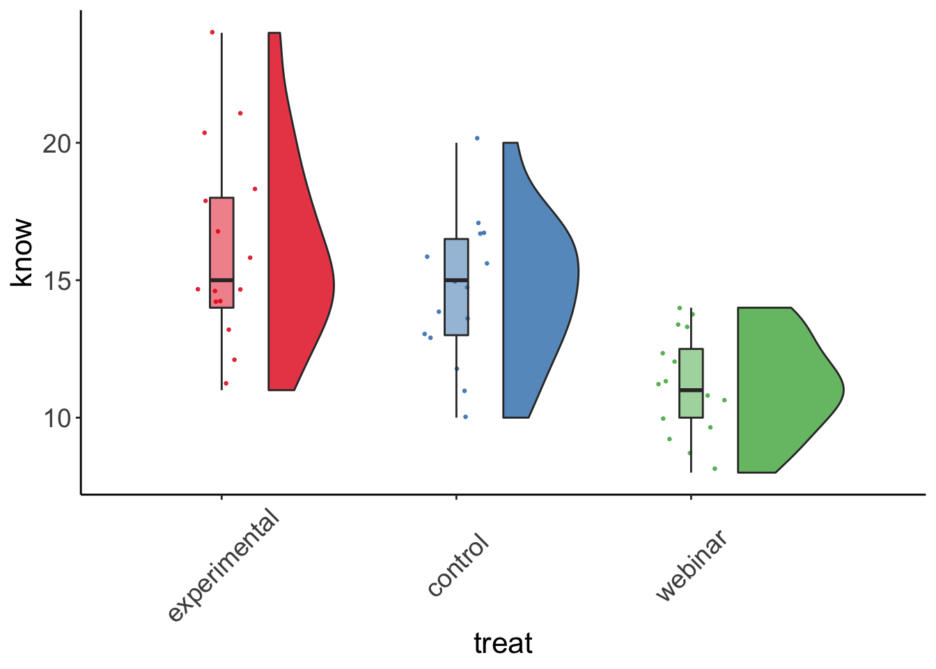

Step 3: Implement MANOVA

Multivariate tests

manova.model2 <- manova(cbind(attitude = attitude, know = know) ~ treat, manova_dat) 
summary(manova.model2, test = "Pillai", intercept=T)

##             Df  Pillai approx F num Df den Df    Pr(>F)    
## (Intercept)  1 0.97196   710.47      2     41 < 2.2e-16 ***
## treat        2 0.91148    17.58      4     84 1.614e-10 ***
## Residuals   42                                             
## ---
## Signif. codes:  0 '***' 0.001 '**' 0.01 '*' 0.05 '.' 0.1 ' ' 1

summary(manova.model2, test = "Wilks", intercept=T)

##             Df    Wilks approx F num Df den Df    Pr(>F)    
## (Intercept)  1 0.028045   710.47      2     41 < 2.2e-16 ***
## treat        2 0.281925    18.11      4     82 1.081e-10 ***
## Residuals   42                                              
## ---
## Signif. codes:  0 '***' 0.001 '**' 0.01 '*' 0.05 '.' 0.1 ' ' 1

summary(manova.model2, test = "Hotelling-Lawley", intercept=T)

##             Df Hotelling-Lawley approx F num Df den Df    Pr(>F)    
## (Intercept)  1           34.657   710.47      2     41 < 2.2e-16 ***
## treat        2            1.861    18.61      4     80 7.589e-11 ***
## Residuals   42                                                      
## ---
## Signif. codes:  0 '***' 0.001 '**' 0.01 '*' 0.05 '.' 0.1 ' ' 1

summary(manova.model2, test = "Roy", intercept=T)

##             Df    Roy approx F num Df den Df    Pr(>F)    
## (Intercept)  1 34.657   710.47      2     41 < 2.2e-16 ***
## treat        2  1.355    28.45      2     42 1.548e-08 ***
## Residuals   42                                            
## ---
## Signif. codes:  0 '***' 0.001 '**' 0.01 '*' 0.05 '.' 0.1 ' ' 1

Box’s M test

library(heplots)

boxtest4 <- boxM(manova_dat[,c("attitude","know")], manova_dat$treat)
summary(boxtest4)

## Summary for Box's M-test of Equality of Covariance Matrices
## 
## Chi-Sq:   9.288089 
## df:   6 
## p-value: 0.158 
## 
## log of Covariance determinants:
## experimental      control      webinar       pooled 
##     4.550595     4.217750     2.509129     3.996638 
## 
## Eigenvalues:
##   experimental control  webinar   pooled
## 1    12.805776 11.4156 5.715718 9.277781
## 2     7.394224  5.9463 2.150949 5.865076
## 
## Statistics based on eigenvalues:
##           experimental   control   webinar    pooled
## product      94.688776 67.880612 12.294218 54.414893
## sum          20.200000 17.361905  7.866667 15.142857
## precision     4.687563  3.909745  1.562824  3.593436
## max          12.805776 11.415604  5.715718  9.277781

Step 4: Follow-up analyses

Univariate ANOVA

aov.att <- aov(attitude~treat, manova_dat)
summary(aov.att)

##             Df Sum Sq Mean Sq F value   Pr(>F)    
## treat        2  424.9  212.47   28.07 1.81e-08 ***
## Residuals   42  317.9    7.57                     
## ---
## Signif. codes:  0 '***' 0.001 '**' 0.01 '*' 0.05 '.' 0.1 ' ' 1

aov.kn <- aov(know~treat, manova_dat)
summary(aov.kn)

##             Df Sum Sq Mean Sq F value   Pr(>F)    
## treat        2  196.8   98.42   12.99 4.05e-05 ***
## Residuals   42  318.1    7.57                     
## ---
## Signif. codes:  0 '***' 0.001 '**' 0.01 '*' 0.05 '.' 0.1 ' ' 1

LSD test

Because the test results for the univariate ANOVA are statistically significant, we can proceed to conducting LSD test for multiple comparisons.

library(agricolae)

lsd.test.att <- LSD.test(aov.att, "treat")
lsd.test.kn <- LSD.test(aov.kn, "treat")

lsd.test.att$groups

##               attitude groups
## control      14.133333      a
## experimental  8.800000      b
## webinar       6.866667      b

lsd.test.kn$groups

##                  know groups
## experimental 16.20000      a
## control      14.66667      a
## webinar      11.20000      b

“Manual” multivariate multiple comparisons

summary(manova(cbind(attitude = attitude, know = know) ~ treat, manova_dat[manova_dat$treat%in%c("experimental","control"),]), test = "Wilks", intercept = T)

##             Df   Wilks approx F num Df den Df    Pr(>F)    
## (Intercept)  1 0.02732   480.57      2     27 < 2.2e-16 ***
## treat        1 0.49391    13.83      2     27 7.316e-05 ***
## Residuals   28                                             
## ---
## Signif. codes:  0 '***' 0.001 '**' 0.01 '*' 0.05 '.' 0.1 ' ' 1

summary(manova(cbind(attitude = attitude, know = know) ~ treat, manova_dat[manova_dat$treat%in%c("experimental","webinar"),]), test = "Wilks", intercept = T)

##             Df   Wilks approx F num Df den Df    Pr(>F)    
## (Intercept)  1 0.03175   411.69      2     27 < 2.2e-16 ***
## treat        1 0.52819    12.06      2     27  0.000181 ***
## Residuals   28                                             
## ---
## Signif. codes:  0 '***' 0.001 '**' 0.01 '*' 0.05 '.' 0.1 ' ' 1

summary(manova(cbind(attitude = attitude, know = know) ~ treat, manova_dat[manova_dat$treat%in%c("webinar","control"),]), test = "Wilks", intercept = T)

##             Df   Wilks approx F num Df den Df    Pr(>F)    
## (Intercept)  1 0.02434   541.23      2     27 < 2.2e-16 ***
## treat        1 0.32864    27.58      2     27 2.991e-07 ***
## Residuals   28                                             
## ---
## Signif. codes:  0 '***' 0.001 '**' 0.01 '*' 0.05 '.' 0.1 ' ' 1

Example 3: Three-group MANOVA with six outcomes

Research Context

The faculties from a public research univeristy were evaluated at the end of a semester with regard to the courses they taught in that semester. Students rated the faculties on six aspects. We are interested in testing whether there is any difference between different types of faculties regarding the set of outcomes.

Step 1: Load the data

library(EDMS657Data)
data(Teacher_ratings)

take a look at the data you just read into R

#View(Teacher_ratings)
glimpse(Teacher_ratings)

## Rows: 120
## Columns: 7
## $ organize <dbl> 4, 7, 6, 6, 4, 8, 2, 4, 4, 6, 7, 7, 4, 5, 5, 5, 3, 6, 7…
## $ clarity  <dbl> 4, 7, 6, 8, 3, 6, 3, 2, 5, 6, 7, 8, 5, 5, 5, 3, 4, 7, 7…
## $ interact <dbl> 3, 6, 5, 6, 5, 8, 3, 2, 6, 6, 4, 6, 4, 6, 4, 5, 5, 5, 7…
## $ workload <dbl> 6, 4, 4, 6, 4, 6, 3, 2, 6, 5, 4, 5, 6, 3, 4, 7, 5, 3, 4…
## $ grading  <dbl> 4, 4, 5, 6, 4, 6, 5, 2, 5, 5, 3, 6, 5, 2, 4, 6, 3, 3, 3…
## $ learning <dbl> 3, 4, 6, 5, 1, 7, 2, 3, 4, 4, 4, 5, 6, 2, 5, 6, 3, 2, 4…
## $ group    <dbl> 1, 1, 1, 1, 1, 1, 1, 1, 1, 1, 1, 1, 1, 1, 1, 1, 1, 1, 1…

str(Teacher_ratings)

## 'data.frame':    120 obs. of  7 variables:
##  $ organize: num  4 7 6 6 4 8 2 4 4 6 ...
##  $ clarity : num  4 7 6 8 3 6 3 2 5 6 ...
##  $ interact: num  3 6 5 6 5 8 3 2 6 6 ...
##  $ workload: num  6 4 4 6 4 6 3 2 6 5 ...
##  $ grading : num  4 4 5 6 4 6 5 2 5 5 ...
##  $ learning: num  3 4 6 5 1 7 2 3 4 4 ...
##  $ group   : num  1 1 1 1 1 1 1 1 1 1 ...
##   ..- attr(*, "value.labels")= Named chr [1:3] "3" "2" "1"
##   .. ..- attr(*, "names")= chr [1:3] "Full" "Associate" "Assistant"
##  - attr(*, "variable.labels")= Named chr [1:7] "course organization and planning" "clarity and communication skills" "teacher/student interaction and rapport" "course difficulty and workload" ...
##   ..- attr(*, "names")= chr [1:7] "organize" "clarity" "interact" "workload" ...
##  - attr(*, "codepage")= int 65001

head(Teacher_ratings)

##   organize clarity interact workload grading learning group
## 1        4       4        3        6       4        3     1
## 2        7       7        6        4       4        4     1
## 3        6       6        5        4       5        6     1
## 4        6       8        6        6       6        5     1
## 5        4       3        5        4       4        1     1
## 6        8       6        8        6       6        7     1

“treatment” is a categorical variable

Teacher_ratings$group <- as.factor(Teacher_ratings$group)
levels(Teacher_ratings$group) <- c("assistant", "associate", "full")

Step 2: Explore the data with descriptive statistics and plots

Descriptive statistics

summary(Teacher_ratings)

##     organize      clarity         interact        workload   
##  Min.   :1.0   Min.   :1.000   Min.   :1.000   Min.   :1.00  
##  1st Qu.:4.0   1st Qu.:4.000   1st Qu.:4.000   1st Qu.:3.00  
##  Median :5.0   Median :5.000   Median :5.000   Median :4.00  
##  Mean   :5.1   Mean   :5.142   Mean   :4.975   Mean   :4.35  
##  3rd Qu.:6.0   3rd Qu.:6.000   3rd Qu.:6.000   3rd Qu.:5.00  
##  Max.   :8.0   Max.   :9.000   Max.   :9.000   Max.   :8.00  
##     grading         learning          group   
##  Min.   :1.000   Min.   :1.00   assistant:40  
##  1st Qu.:3.000   1st Qu.:3.00   associate:40  
##  Median :4.000   Median :4.00   full     :40  
##  Mean   :4.225   Mean   :4.45                 
##  3rd Qu.:5.000   3rd Qu.:5.00                 
##  Max.   :9.000   Max.   :9.00

table(Teacher_ratings$group)

## 
## assistant associate      full 
##        40        40        40

Within-group means

for (i in 1:6){
  print(colnames(Teacher_ratings)[i])
  print(with(Teacher_ratings, tapply(Teacher_ratings[,i], group, mean)))
}

## [1] "organize"
## assistant associate      full 
##     5.075     5.725     4.500 
## [1] "clarity"
## assistant associate      full 
##     5.200     5.875     4.350 
## [1] "interact"
## assistant associate      full 
##     4.875     5.750     4.300 
## [1] "workload"
## assistant associate      full 
##      4.40      5.00      3.65 
## [1] "grading"
## assistant associate      full 
##     4.125     5.025     3.525 
## [1] "learning"
## assistant associate      full 
##     4.275     5.250     3.825

Within-group variances

for (i in 1:6){
  print(colnames(Teacher_ratings)[i])
  print(with(Teacher_ratings, tapply(Teacher_ratings[,i], group, var)))
}

## [1] "organize"
## assistant associate      full 
##  3.096795  1.896795  1.948718 
## [1] "clarity"
## assistant associate      full 
##  2.882051  1.958333  2.130769 
## [1] "interact"
## assistant associate      full 
##  2.727564  2.397436  2.830769 
## [1] "workload"
## assistant associate      full 
##  2.451282  3.333333  1.156410 
## [1] "grading"
## assistant associate      full 
##  1.548077  2.486538  1.025000 
## [1] "learning"
## assistant associate      full 
## 2.2044872 2.5000000 0.9685897

Descriptive plots

Let’s try something different from the previous two examples. The following plot shows the covariance ellipse for each group.

library(heplots)
covEllipses(Teacher_ratings[,1:6], Teacher_ratings$group, 
            fill=c(rep(FALSE,3), TRUE), pooled=F)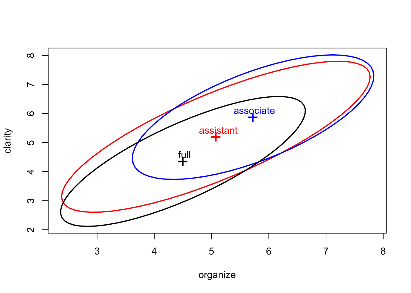

You can center the covariance ellipses by setting a common centroid for all the groups.

covEllipses(Teacher_ratings[,1:6], Teacher_ratings$group, center=TRUE, fill=c(rep(FALSE,3), TRUE), fill.alpha=.1, label.pos=c(1:3,0), pooled=F)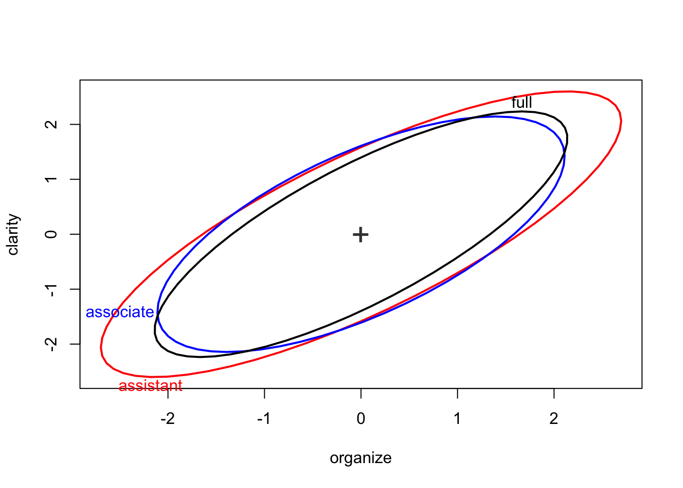

We can even add the pooled covariance ellipse, centered or uncentered.

covEllipses(Teacher_ratings[,1:6], Teacher_ratings$group, 
            fill=c(rep(FALSE,3), TRUE))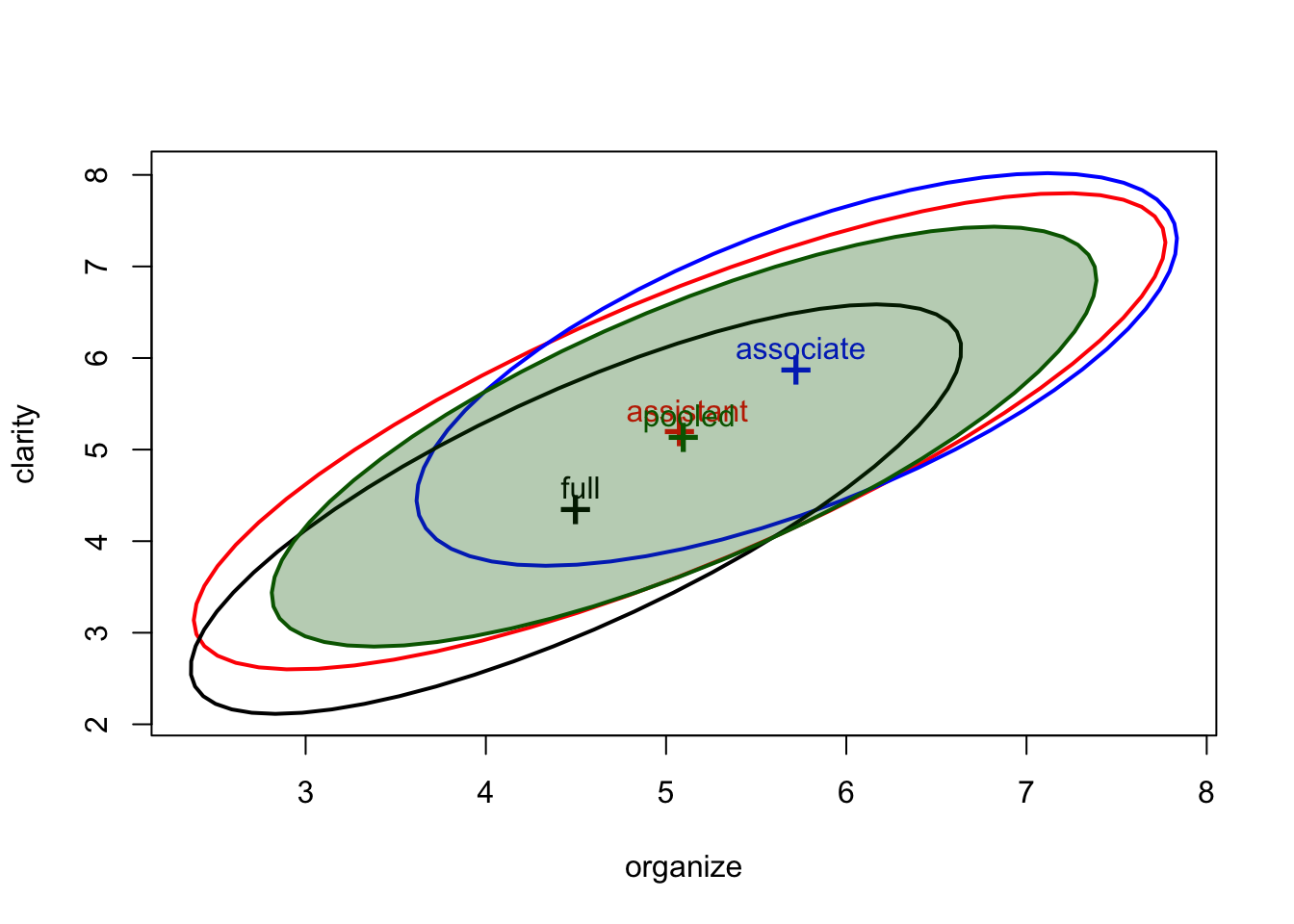

covEllipses(Teacher_ratings[,1:6], Teacher_ratings$group,center=TRUE, fill=c(rep(FALSE,3), TRUE), fill.alpha=.1, label.pos=c(1:3,0))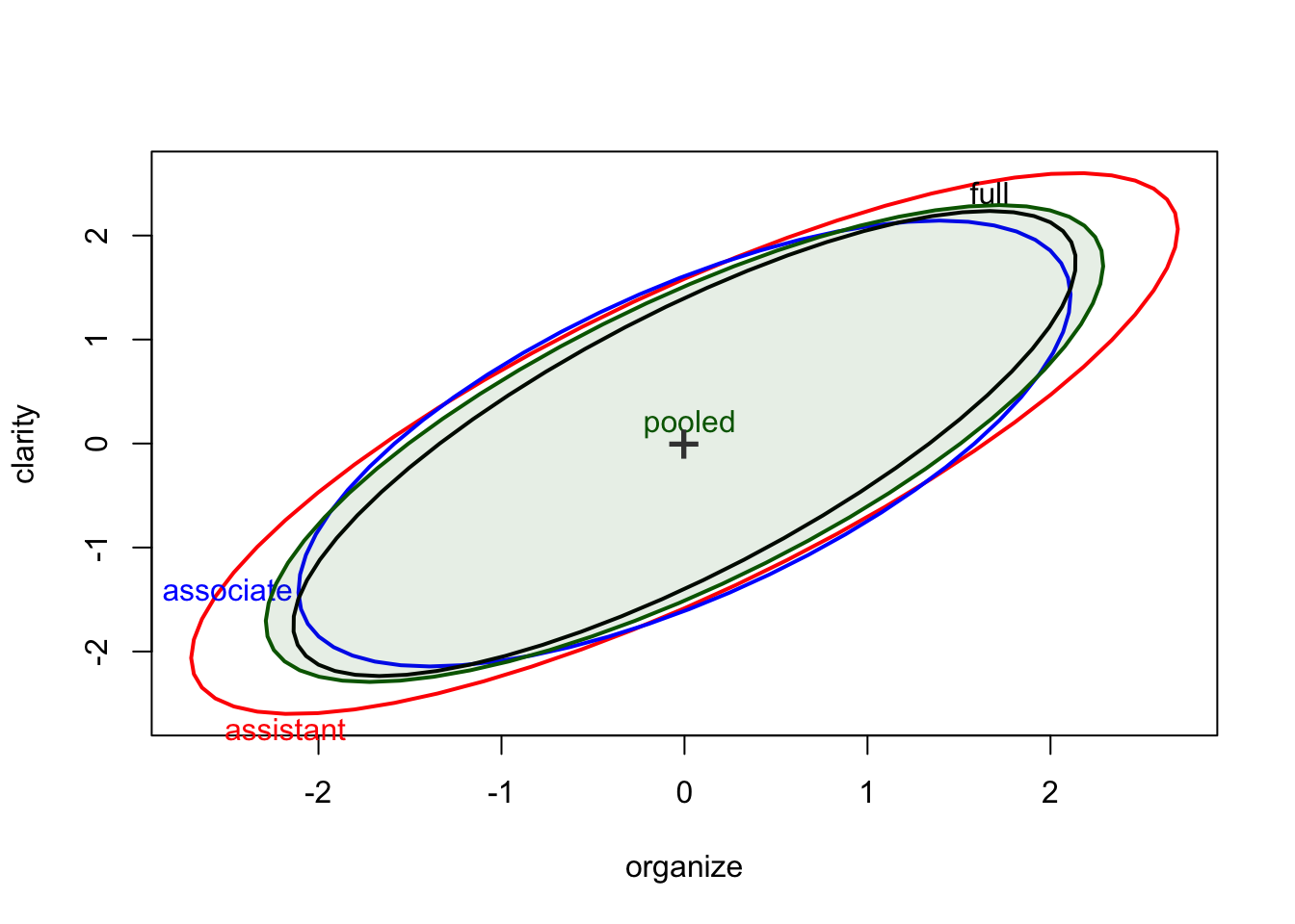

Let’s see the covariances between all possible pairs of the variables.

covEllipses(Teacher_ratings[,1:6], Teacher_ratings$group, 
            fill=c(rep(FALSE,3), TRUE), variables=1:6, 
            fill.alpha=.1,pooled=F)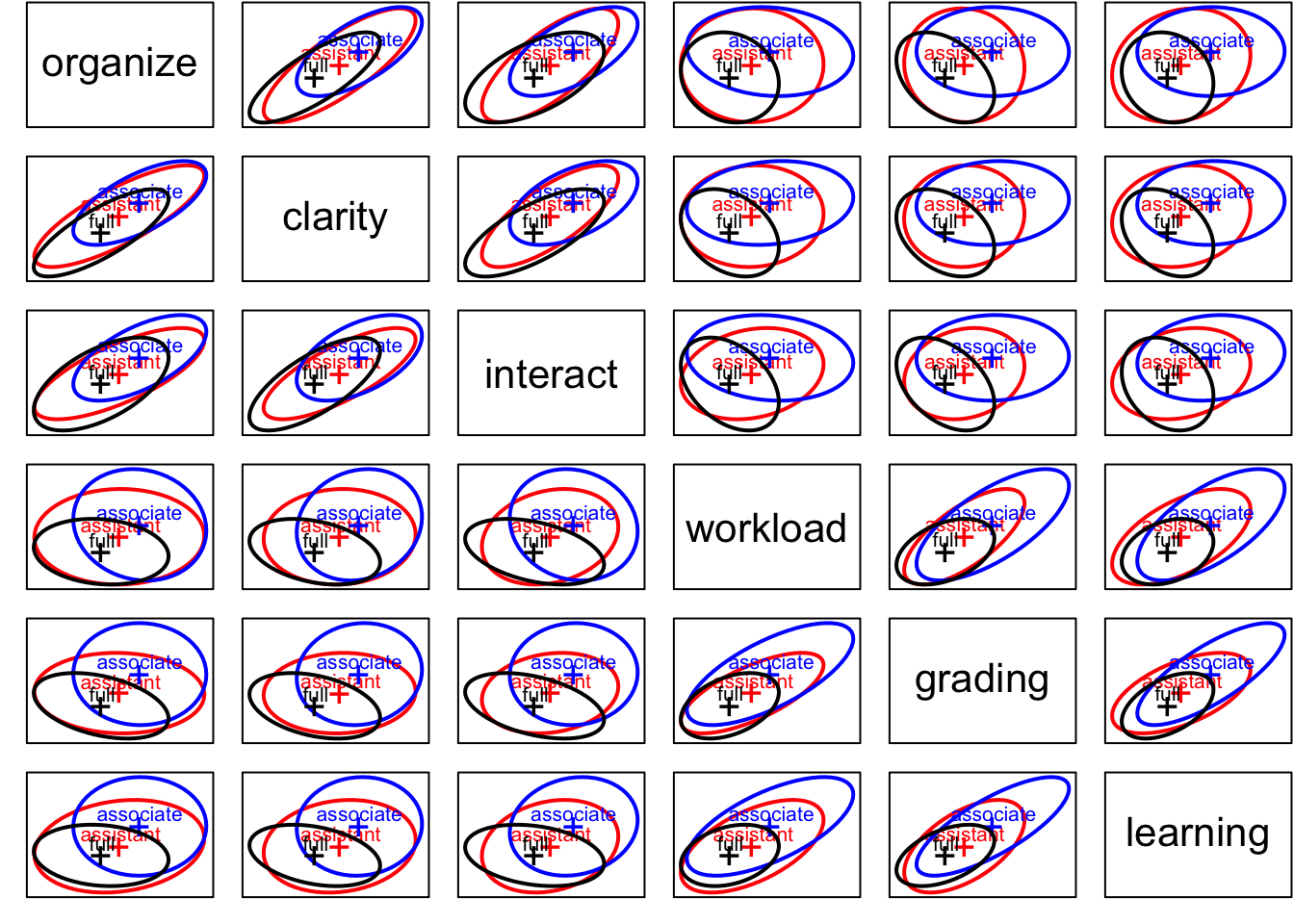

covEllipses(Teacher_ratings[,1:6], Teacher_ratings$group, center=T, fill=c(rep(FALSE,3), TRUE), variables=1:6, 
            fill.alpha=.1,pooled=F)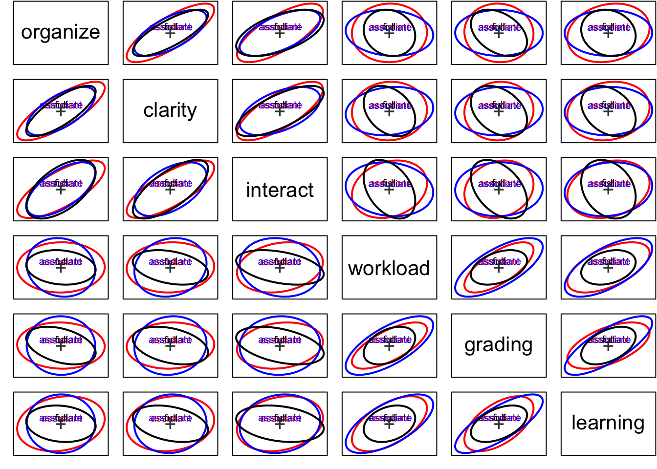

We can also view the data points in principal components space.

manova.data3.pca <- prcomp(Teacher_ratings[,1:6])
summary(manova.data3.pca)

## Importance of components:
##                           PC1    PC2     PC3     PC4     PC5     PC6
## Standard deviation     2.6597 2.2185 1.02483 0.92508 0.80284 0.68122
## Proportion of Variance 0.4713 0.3279 0.06997 0.05701 0.04294 0.03092
## Cumulative Proportion  0.4713 0.7992 0.86913 0.92614 0.96908 1.00000

op <- par(mfcol=c(1,2), mar=c(5,4,1,1)+.1)

covEllipses(manova.data3.pca$x, Teacher_ratings$group, 
            fill=c(rep(FALSE,3), TRUE), 
            label.pos=1:4, fill.alpha=.1, asp=1,pooled=F)

covEllipses(manova.data3.pca$x, Teacher_ratings$group, 
            fill=c(rep(FALSE,3), TRUE), variables=3:4,
            label.pos=1:4, fill.alpha=.1, asp=1,pooled=F)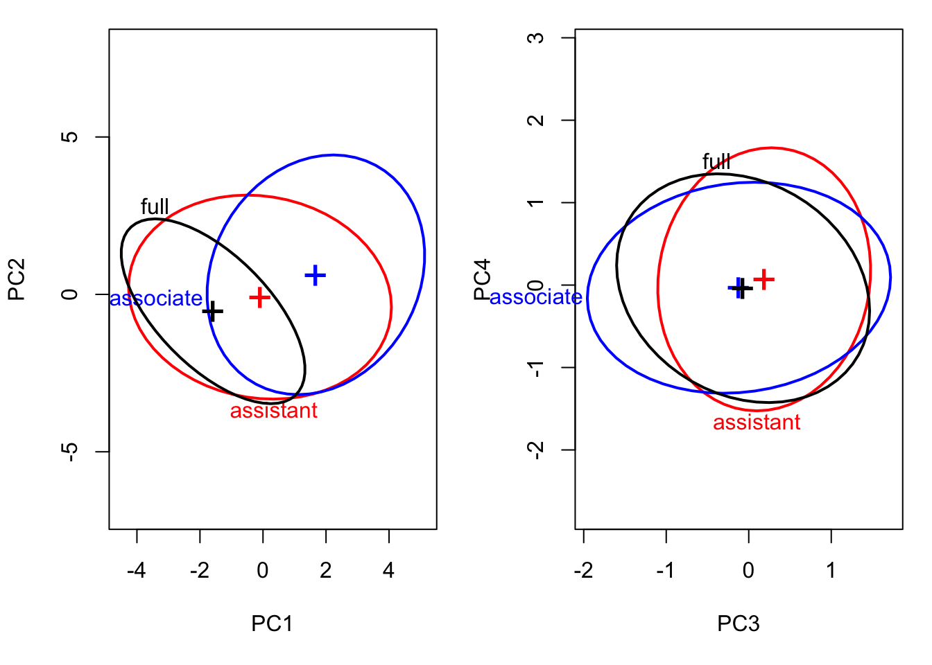

covEllipses(manova.data3.pca$x, Teacher_ratings$group, 
            fill=c(rep(FALSE,3), TRUE), variables=1:6,
            label.pos=1:4, fill.alpha=.1, asp=1,pooled=F)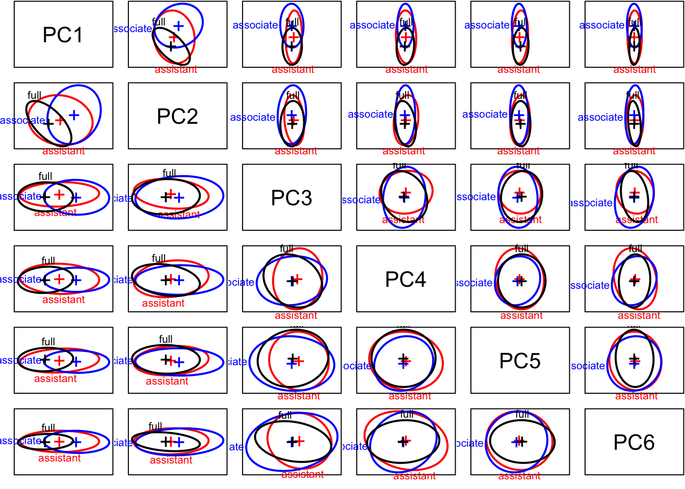

par(op)

Step 3: Implement MANOVA

Multivariate tests

manova.model3 <- manova(cbind(organize, clarity, interact, workload, grading,  learning) ~ group, Teacher_ratings)
summary(manova.model3, test = "Pillai", intercept=T)

##              Df  Pillai approx F num Df den Df    Pr(>F)    
## (Intercept)   1 0.96611   532.21      6    112 < 2.2e-16 ***
## group         2 0.33405     3.78     12    226 3.086e-05 ***
## Residuals   117                                             
## ---
## Signif. codes:  0 '***' 0.001 '**' 0.01 '*' 0.05 '.' 0.1 ' ' 1

summary(manova.model3, test = "Wilks", intercept=T)

##              Df   Wilks approx F num Df den Df    Pr(>F)    
## (Intercept)   1 0.03389   532.21      6    112 < 2.2e-16 ***
## group         2 0.67235     4.10     12    224 8.686e-06 ***
## Residuals   117                                             
## ---
## Signif. codes:  0 '***' 0.001 '**' 0.01 '*' 0.05 '.' 0.1 ' ' 1

summary(manova.model3, test = "Hotelling-Lawley", intercept=T)

##              Df Hotelling-Lawley approx F num Df den Df    Pr(>F)    
## (Intercept)   1          28.5113   532.21      6    112 < 2.2e-16 ***
## group         2           0.4778     4.42     12    222 2.452e-06 ***
## Residuals   117                                                      
## ---
## Signif. codes:  0 '***' 0.001 '**' 0.01 '*' 0.05 '.' 0.1 ' ' 1

summary(manova.model3, test = "Roy", intercept=T)

##              Df    Roy approx F num Df den Df    Pr(>F)    
## (Intercept)   1 28.511   532.21      6    112 < 2.2e-16 ***
## group         2  0.457     8.61      6    113 1.038e-07 ***
## Residuals   117                                            
## ---
## Signif. codes:  0 '***' 0.001 '**' 0.01 '*' 0.05 '.' 0.1 ' ' 1

Box’s M test

library(heplots)

boxtest6 <- boxM(Teacher_ratings[,1:6], Teacher_ratings$group)
summary(boxtest6)

## Summary for Box's M-test of Equality of Covariance Matrices
## 
## Chi-Sq:   56.1123 
## df:   42 
## p-value: 0.07135 
## 
## log of Covariance determinants:
##   assistant   associate        full      pooled 
##  2.05352330  2.25782486 -0.03899053  1.94116978 
## 
## Eigenvalues:
##   assistant associate      full    pooled
## 1 7.5445874 6.6965430 5.9976581 5.7899999
## 2 4.4509180 4.5908871 1.4803104 4.3594037
## 3 1.1212748 1.4661925 1.0181861 1.0496581
## 4 0.6645808 0.7631897 0.6961131 0.8676318
## 5 0.6485849 0.5527171 0.6224494 0.6427895
## 6 0.4803105 0.5029064 0.2455394 0.4714999
## 
## Statistics based on eigenvalues:
##            assistant  associate       full     pooled
## product    7.7953180  9.5622673  0.9617598  6.9668960
## sum       14.9102564 14.5724359 10.0602564 13.1809829
## precision  0.1567995  0.1624123  0.1118546  0.1617085
## max        7.5445874  6.6965430  5.9976581  5.7899999

Step 4: Follow-up analyses

Univariate ANOVA

anova(lm(organize~group, Teacher_ratings))

## Analysis of Variance Table
## 
## Response: organize
##            Df Sum Sq Mean Sq F value   Pr(>F)   
## group       2  30.05 15.0250  6.4928 0.002118 **
## Residuals 117 270.75  2.3141                    
## ---
## Signif. codes:  0 '***' 0.001 '**' 0.01 '*' 0.05 '.' 0.1 ' ' 1

anova(lm(clarity~group,  Teacher_ratings))

## Analysis of Variance Table
## 
## Response: clarity
##            Df  Sum Sq Mean Sq F value    Pr(>F)    
## group       2  46.717 23.3583  10.052 9.362e-05 ***
## Residuals 117 271.875  2.3237                      
## ---
## Signif. codes:  0 '***' 0.001 '**' 0.01 '*' 0.05 '.' 0.1 ' ' 1

anova(lm(interact~group, Teacher_ratings))

## Analysis of Variance Table
## 
## Response: interact
##            Df Sum Sq Mean Sq F value    Pr(>F)    
## group       2  42.65 21.3250  8.0413 0.0005343 ***
## Residuals 117 310.27  2.6519                      
## ---
## Signif. codes:  0 '***' 0.001 '**' 0.01 '*' 0.05 '.' 0.1 ' ' 1

anova(lm(workload~group, Teacher_ratings))

## Analysis of Variance Table
## 
## Response: workload
##            Df Sum Sq Mean Sq F value Pr(>F)    
## group       2   36.6 18.3000  7.9095  6e-04 ***
## Residuals 117  270.7  2.3137                   
## ---
## Signif. codes:  0 '***' 0.001 '**' 0.01 '*' 0.05 '.' 0.1 ' ' 1

anova(lm(grading~group,  Teacher_ratings))

## Analysis of Variance Table
## 
## Response: grading
##            Df Sum Sq Mean Sq F value    Pr(>F)    
## group       2  45.60 22.8000  13.519 5.224e-06 ***
## Residuals 117 197.32  1.6865                      
## ---
## Signif. codes:  0 '***' 0.001 '**' 0.01 '*' 0.05 '.' 0.1 ' ' 1

anova(lm(learning~group, Teacher_ratings))

## Analysis of Variance Table
## 
## Response: learning
##            Df Sum Sq Mean Sq F value    Pr(>F)    
## group       2  42.45  21.225  11.224 3.473e-05 ***
## Residuals 117 221.25   1.891                      
## ---
## Signif. codes:  0 '***' 0.001 '**' 0.01 '*' 0.05 '.' 0.1 ' ' 1

Tukey’s HSD test

library(agricolae)

(HSD.test(aov(organize~group, Teacher_ratings), "group"))$groups

##           organize groups
## associate    5.725      a
## assistant    5.075     ab
## full         4.500      b

(HSD.test(aov(clarity~group,  Teacher_ratings), "group"))$groups

##           clarity groups
## associate   5.875      a
## assistant   5.200      a
## full        4.350      b

(HSD.test(aov(interact~group, Teacher_ratings), "group"))$groups

##           interact groups
## associate    5.750      a
## assistant    4.875      b
## full         4.300      b

(HSD.test(aov(workload~group, Teacher_ratings), "group"))$groups

##           workload groups
## associate     5.00      a
## assistant     4.40     ab
## full          3.65      b

(HSD.test(aov(grading~group,  Teacher_ratings), "group"))$groups

##           grading groups
## associate   5.025      a
## assistant   4.125      b
## full        3.525      b

(HSD.test(aov(learning~group, Teacher_ratings), "group"))$groups

##           learning groups
## associate    5.250      a
## assistant    4.275      b
## full         3.825      b

“Manual” multivariate multiple comparisons

summary(manova(cbind(organize, clarity, interact, workload, grading, learning) ~ group, Teacher_ratings[Teacher_ratings$group %in% c("assistant","associate"), ]), intercept = T)

##             Df  Pillai approx F num Df den Df  Pr(>F)    
## (Intercept)  1 0.96255  312.683      6     73 < 2e-16 ***
## group        1 0.15791    2.282      6     73 0.04494 *  
## Residuals   78                                           
## ---
## Signif. codes:  0 '***' 0.001 '**' 0.01 '*' 0.05 '.' 0.1 ' ' 1

summary(manova(cbind(organize, clarity, interact, workload, grading, learning) ~ group, Teacher_ratings[Teacher_ratings$group %in% c("assistant","full"),]), intercept = T)

##             Df  Pillai approx F num Df den Df  Pr(>F)    
## (Intercept)  1 0.96638   349.77      6     73 < 2e-16 ***
## group        1 0.16240     2.36      6     73 0.03876 *  
## Residuals   78                                           
## ---
## Signif. codes:  0 '***' 0.001 '**' 0.01 '*' 0.05 '.' 0.1 ' ' 1

summary(manova(cbind(organize, clarity, interact, workload, grading,  learning) ~ group, Teacher_ratings[Teacher_ratings$group %in% c("full","associate"),]), intercept = T)

##             Df  Pillai approx F num Df den Df    Pr(>F)    
## (Intercept)  1 0.97224   426.17      6     73 < 2.2e-16 ***
## group        1 0.44391     9.71      6     73 7.584e-08 ***
## Residuals   78                                             
## ---
## Signif. codes:  0 '***' 0.001 '**' 0.01 '*' 0.05 '.' 0.1 ' ' 1

Discriminant function analysis (Canonical discrimination analysis/linear discriminant analysis)

library(candisc)

disc <- candisc(manova(cbind(organize, clarity, interact, workload, grading, learning) ~ group, Teacher_ratings))
summary(disc, scores = F)

## 
## Canonical Discriminant Analysis for group:
## 
##     CanRsq Eigenvalue Difference Percent Cumulative
## 1 0.313654    0.45699    0.43617 95.6427     95.643
## 2 0.020395    0.02082    0.43617  4.3573    100.000
## 
## Class means:
## 
##                Can1      Can2
## assistant -0.068936  0.200953
## associate  0.849812 -0.087734
## full      -0.780876 -0.113219
## 
##  std coefficients:
##              Can1     Can2
## organize 0.094533 -0.19892
## clarity  0.400276  0.85437
## interact 0.238116 -0.47068
## workload 0.084000  0.86171
## grading  0.550587 -0.25997
## learning 0.223505 -0.68948

Wilks’ Lambda

Wilks(disc)

## 
## Test of H0: The canonical correlations in the 
## current row and all that follow are zero
## 
##   LR test stat approx F numDF denDF   Pr(> F)    
## 1      0.67235   4.0984    12   224 8.686e-06 ***
## 2      0.97960   0.4705     5   113    0.7975    
## ---
## Signif. codes:  0 '***' 0.001 '**' 0.01 '*' 0.05 '.' 0.1 ' ' 1

Structure coefficients

disc$structure

##               Can1       Can2
## organize 0.5639597  0.0835453
## clarity  0.6771253  0.3721678
## interact 0.6200649 -0.1114412
## workload 0.6104303  0.3303997
## grading  0.7729296 -0.1269871
## learning 0.7097412 -0.3822816

coef(disc, type = "structure")

##               Can1       Can2
## organize 0.5639597  0.0835453
## clarity  0.6771253  0.3721678
## interact 0.6200649 -0.1114412
## workload 0.6104303  0.3303997
## grading  0.7729296 -0.1269871
## learning 0.7097412 -0.3822816

Plot the discriminant function space

plot(disc, which = 1:2, conf = 0.95,asp = 1, scale=4,
     var.col = "blue", var.lwd = par("lwd"),  var.cex = 1,
     rev.axes=c(FALSE, FALSE),
     ellipse=FALSE, ellipse.prob = 0.68, fill.alpha=0.1,
     prefix = "DF", suffix=TRUE,
     titles.1d = c("Canonical scores", "Structure"))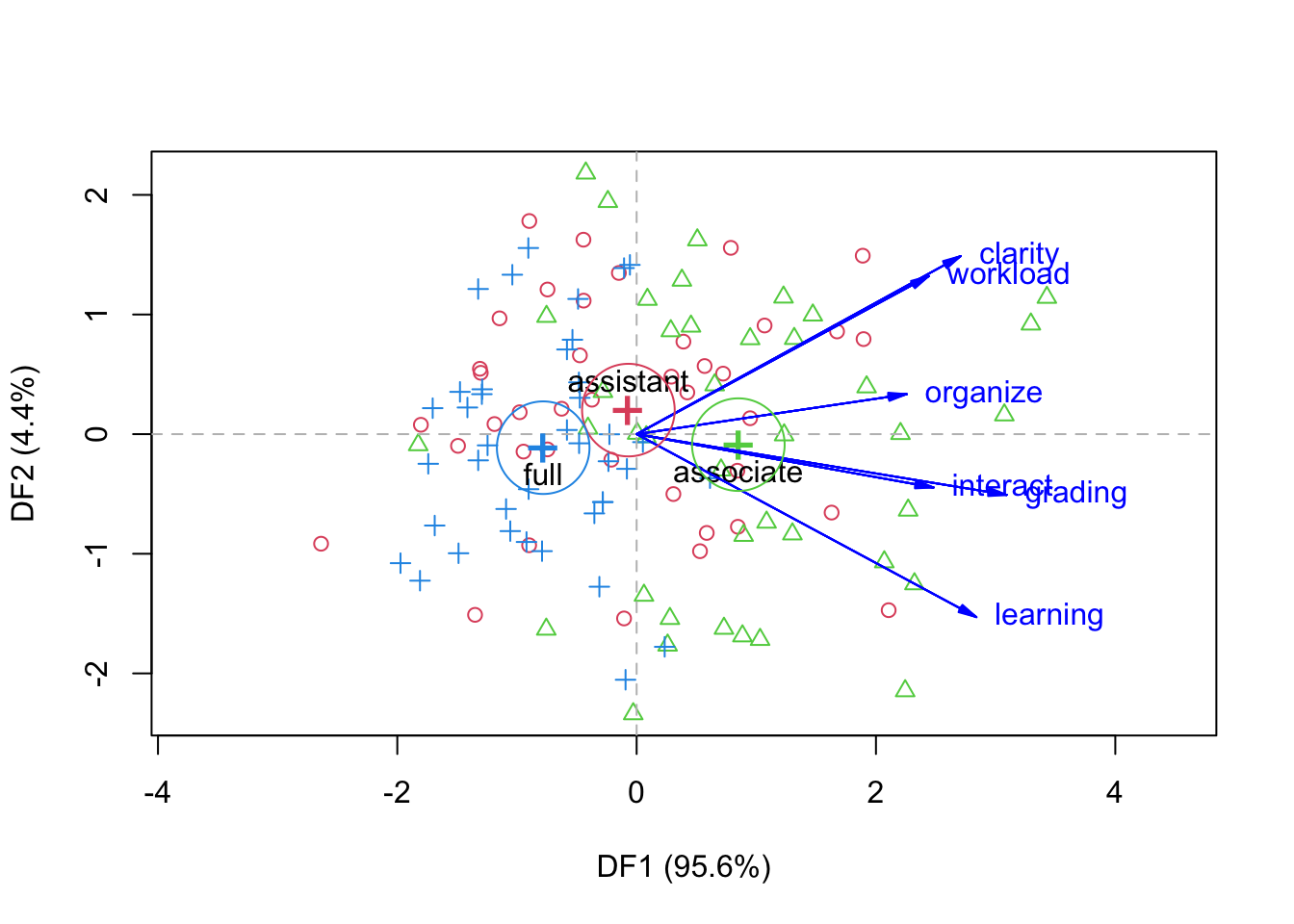

Examine the distribution of LDA scores

Teacher_ratings$lda1 <- disc$scores[,2]
Teacher_ratings$lda2 <- disc$scores[,3]

ggplot(Teacher_ratings, aes(lda1, fill =group)) + geom_density(alpha = 0.5, color = NA) + theme(legend.position = "top")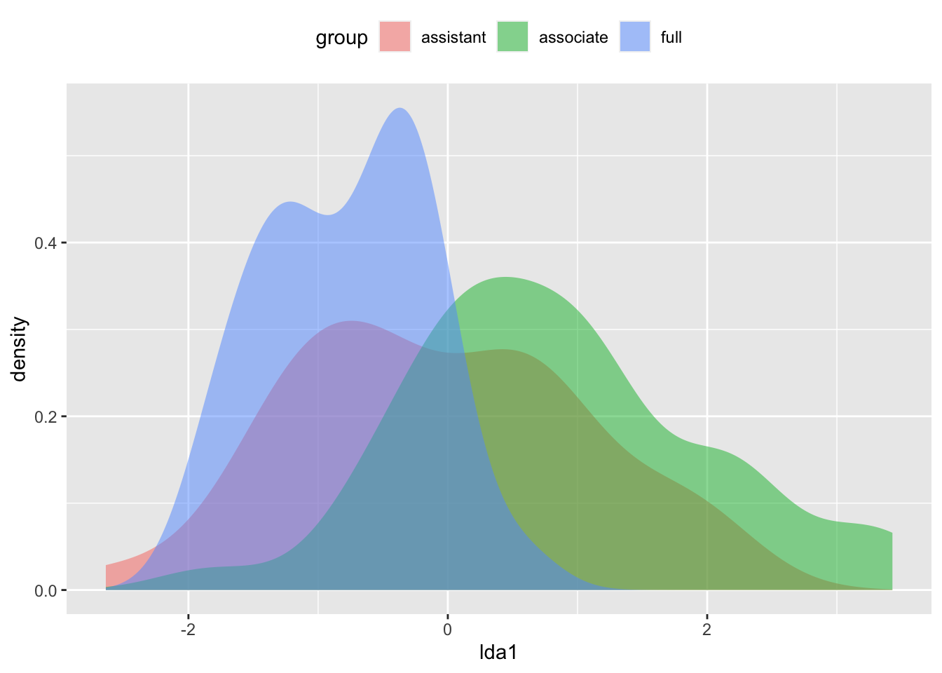

ggplot(Teacher_ratings, aes(lda2, fill =group)) + geom_density(alpha = 0.5, color = NA) + theme(legend.position = "top")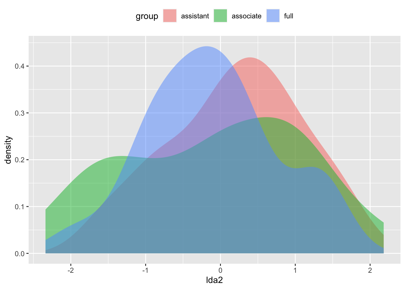

rc_plot3 <- ggplot(data = Teacher_ratings, aes(x=group, y=lda1, fill = group)) +
geom_flat_violin(position = position_nudge(x = .2, y = 0), alpha = .8) +
geom_point(aes(y=lda1, color = group), position = position_jitter(width = .15), size = .5, alpha = 0.8) +
geom_boxplot(width = .1, guides = FALSE, outlier.shape = NA, alpha = 0.5) +
expand_limits(x = 4, y = 4) +
ylab("First Discriminant Function") +
guides(fill = FALSE) +
guides(color = FALSE) +
scale_color_brewer(palette = "Set1") +
scale_fill_brewer(palette = "Set1") +
theme_bw() +
raincloud_theme

rc_plot3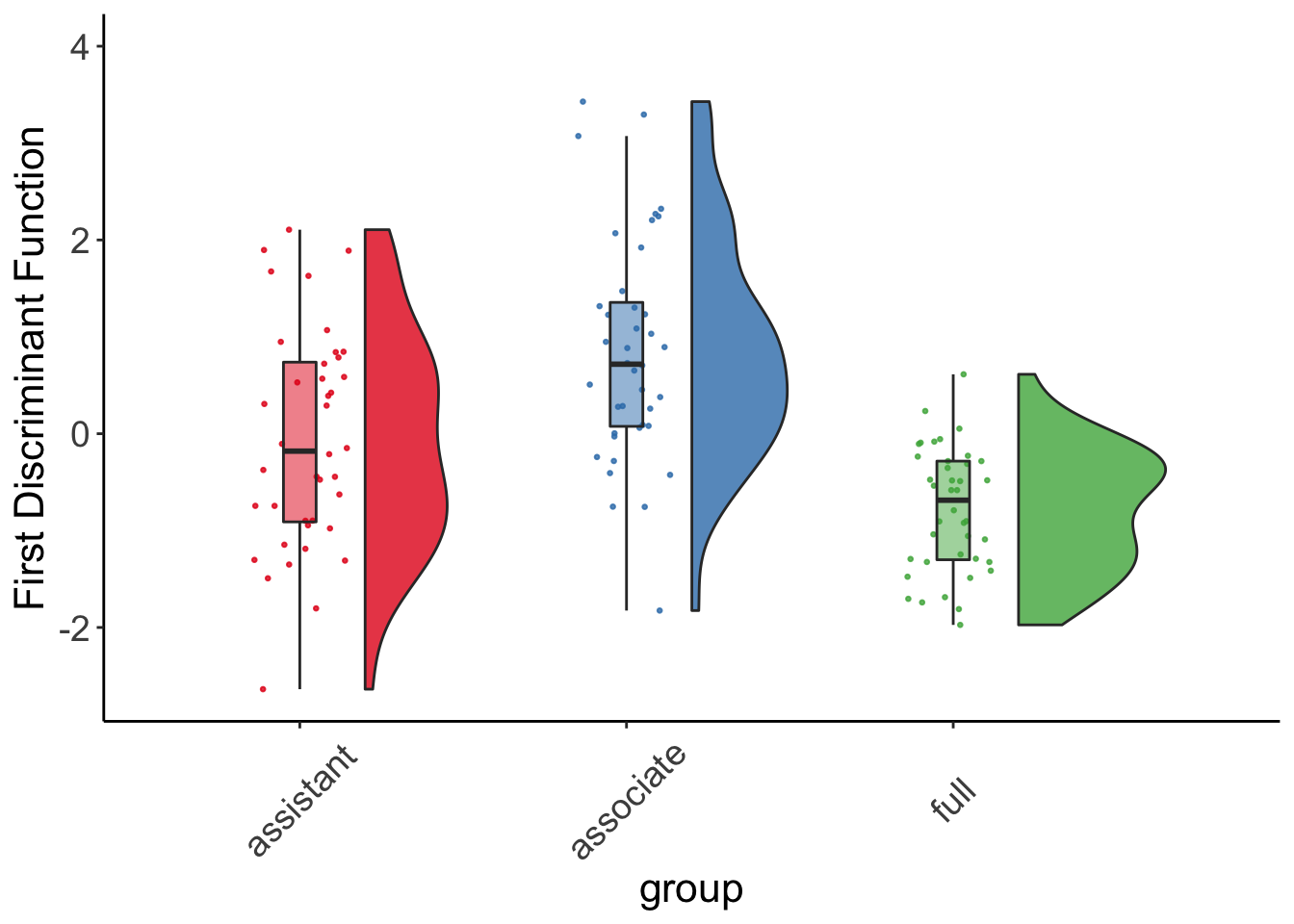

The R script for this tutorial can be found here.

EDMS 657-R Tutorial: MANOVA

Yi Feng & Gregory R. Hancock

Example 1: Two-group MANOVA / Hoteling’s \(T^2\)

Step 1: Read and examine the data

Load the data into the R session.

Take a look at the data

Step 2: Explore the data with descriptive statistics and plots

Descriptive statistics

Descriptive plots

Step 3: Implement MANOVA analysis

Multivariate tests

Step 4: Follow-up: Univariate ANOVA

Example 2: Three-group MANOVA

Step 1: Load the data

take a look at the data you just read into R

Step 2: Explore the data with descriptive statistics and plots

Descriptive statistics

Within-group means

Within-group variances

Descriptive plots

Scatterplot

Add centroids

Boxplots

Raincloud plots

Step 3: Implement MANOVA

Multivariate tests

Box’s M test

Step 4: Follow-up analyses

Univariate ANOVA

LSD test

“Manual” multivariate multiple comparisons

Example 3: Three-group MANOVA with six outcomes

Step 1: Load the data

take a look at the data you just read into R

“treatment” is a categorical variable

Step 2: Explore the data with descriptive statistics and plots

Descriptive statistics

Within-group means

Within-group variances

Descriptive plots

Step 3: Implement MANOVA

Multivariate tests

Box’s M test

Step 4: Follow-up analyses

Univariate ANOVA

Tukey’s HSD test

“Manual” multivariate multiple comparisons

Discriminant function analysis (Canonical discrimination analysis/linear discriminant analysis)