EDMS 657-R Tutorial: Latent Class Analysis
Yi Feng
EDMS, University of MarylandFirst, let’s install the R package to be used for this LCA example.
install.packages("poLCA")
devtools::install_github("YiFengEDMS/EDMS657Data")
Load Data
Next let’s load the data into the R environment and get some descriptive statistics for the data.
This data example consists of three variables, recording the item responses for three questions asking students about thier cheating behaviors.
Dayton & Scheers (1997) surveyed n=319 upper level undergraduates about their cheating behavior in the university setting. * “Have you ever lied to avoid taking an exam and/or to avoid handing in a paper on time?” (x) * “Have you ever purchased a term paper and/or acquired a copy of an exam ahead of time?” (y) * “Have you ever copied answers from another student during an exam?” (z)
library(EDMS657Data)
data(cheat_dat)

head(cheat_dat)
## x y z
## 1 0 0 0
## 2 0 0 0
## 3 1 0 0
## 4 0 0 0
## 5 0 0 0
## 6 1 0 1table(cheat_dat$x, cheat_dat$y, cheat_dat$z)## , , = 0
##
##
## 0 1
## 0 207 7
## 1 46 5
##
## , , = 1
##
##
## 0 1
## 0 34 3
## 1 11 6Fit a LCA Model
We will use the poLCA package to fit the LCA model.
Because poLCA requires data values starting at 1, we will
first transform the data by turning the binary values to (1, 2) in place
of (0, 1).
We first fit a model with two latent classes.
library(poLCA)

cheat_dat <- cheat_dat + 1

f <- with(cheat_dat, cbind(x, y, z) ~ 1)
lc2 <- poLCA(formula = f, cheat_dat, nclass = 2)  # two latent classes
## Conditional item response (column) probabilities,
## by outcome variable, for each class (row)
##
## $x
## Pr(1) Pr(2)
## class 1: 0.8265 0.1735
## class 2: 0.2668 0.7332
##
## $y
## Pr(1) Pr(2)
## class 1: 0.9735 0.0265
## class 2: 0.4183 0.5817
##
## $z
## Pr(1) Pr(2)
## class 1: 0.8638 0.1362
## class 2: 0.3966 0.6034
##
## Estimated class population shares
## 0.9292 0.0708
##
## Predicted class memberships (by modal posterior prob.)
## 0.9561 0.0439
##
## =========================================================
## Fit for 2 latent classes:
## =========================================================
## number of observations: 319
## number of estimated parameters: 7
## residual degrees of freedom: 0
## maximum log-likelihood: -377.1176
##
## AIC(2): 768.2352
## BIC(2): 794.5916
## G^2(2): 2.166167e-09 (Likelihood ratio/deviance statistic)
## X^2(2): 2.167377e-09 (Chi-square goodness of fit)
## You could check out the predicted class membership for each observation:
cheat.predclass <- cbind(cheat_dat - 1, "Predicted Class" = lc2$predclass)

head(cheat.predclass)
## x y z Predicted Class
## 1 0 0 0 1
## 2 0 0 0 1
## 3 1 0 0 1
## 4 0 0 0 1
## 5 0 0 0 1
## 6 1 0 1 1Model Comparison
We could fit a series of models with different numbers of latent classes and compare the model fit across different models.
I will use a user-defined function for this task, which will run a series of models and summarize the model fit indices for each of the models:
LCA_fit <- function(nk, data, nrep){

lc_bic <- rep(NA, length(nk))
lc_model <- list(length = length(nk))

# summarize the results in a table
summary_table <- matrix (NA, nrow = length(nk), ncol = 7)
colnames(summary_table) <- c("Model", "log_likelihood", "df", "BIC", "ABIC", "CAIC", "likelihood_ratio")


for(i in nk){
  lc <- poLCA(f, data = data, nclass=i, maxiter=3000,
              tol=1e-5, na.rm=FALSE,
              nrep = nrep, verbose=TRUE, calc.se=TRUE)
  lc_bic[i] <- lc$bic
  lc_model[[i]] <- lc

  summary_table[i,1] <- paste0("Model ", i)
  summary_table[i,2] <- lc$llik
  summary_table[i,3] <- lc$resid.df
  summary_table[i,4] <- lc$bic
  summary_table[i,5] <- (-2*lc$llik) + ((log((lc$N + 2)/24)) * lc$npar)
  summary_table[i,6] <- (-2*lc$llik) + lc$npar * (1 + log(lc$N))
  summary_table[i,7] <- lc$Gsq

}

best_model <- lc_model[[which.min(lc_bic)]]
summary_table <- as.data.frame(summary_table)
summary_table[, 2:7] <- apply(summary_table[, 2:7], 2, as.numeric)


results <- list(lc_bic, lc_model, best_model, summary_table)
names(results) <- c("BIC", "Models", "Best Model", "Results")
return(results)

}
Now I can use the function defined above to fit two different models to the data, with one to two latent classes respectively. We could certainly fit models with more than two latent classes using the same function if we have a different data example.
lca_models <- LCA_fit(1:2, data = cheat_dat, nrep = 10)lca_models$Results## Model log_likelihood df BIC ABIC CAIC likelihood_ratio
## 1 Model 1 -387.7703 4 792.8362 783.3208 795.8362 21.305387800
## 2 Model 2 -377.1177 0 794.5917 772.3891 801.5917 0.000190113You could plot certain fit index (e.g., BIC) across different models. Again, this may be more useful when you have a number of different models to compare.
plot(1:2, lca_models$Results$ABIC, type = "b", xlab = "Number of Latent Classes", ylab = "ABIC", col = "darkred", xaxt="n")
axis(1, at = seq(1, 2, by = 1))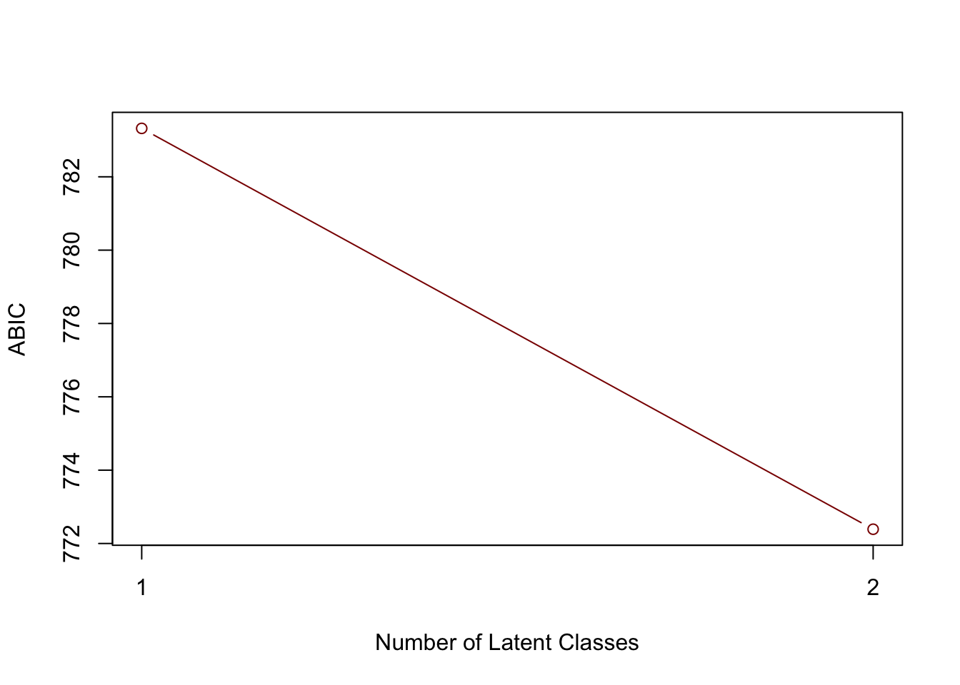
Entropy Measure
A summary measure of classification for LCA is the entropy measure. The entropy formula used by Mplus is given in its technical appendix 8 (Eq. 171).
\[E_k = 1 - \frac{\sum_i\sum_k(-p_{ik}\text{ ln}p_{ik})}{n\text{ ln}K}\] where \(p_{ik}\) is estimated probability of observation \(i\) in latent class\(k\). Based on this formula, entropy values ranges from 0 to 1, with a value closer to 1 indicating clearer classification between the latent classes.
Again, I’m going to define a function to compute entropy based on the LCA model output:
entropy <- function(posterior){

  n <- nrow(posterior)
  k <- ncol(posterior)

  val <- 0

  for (i in 1:n){
    for(j in 1:k){
      val <- val - posterior[i,k]*ifelse(posterior[i,k]==0, 0, log(posterior[i,k]))
    }
  }

  entrp <- 1 - val/(n*log(k))

  return(entrp)

}
Now we can compute the entropy measure for the LCA model we just fit with two latent classes:
entropy(lc2$posterior)## [1] 0.7644238The R script for this tutorial can be found here.
© Copyright 2022 Yi Feng and Gregory R. Hancock.