EDMS 657-R Tutorial: Exploratory Factor Analysis
Yi Feng & Gregory R. Hancock
University of Maryland, College ParkIn this document we demonstrate some examples of factor analysis using R, mainly focusing on principal axis factoring (PAF). This document serves as a supplementary material for EDMS 657-Exploratory Latent and Composite Variable Methods, taught by Dr. Gregory R. Hancock at University of Maryland.
Before we get started, let’s make sure we install and load all the packages we need to use in this demo.
install.packages("psych")
devtools::install_github("YiFengEDMS/EDMS657Data")
library(psych)
library(EDMS657Data)
PAF Example 1: Analyzing Spearman’s data using PAF
1. Prepare data
In this example, we are using a correlation matrix as the input data.
spearman## XC XF XE XM XP XT
## XC 1.00 0.83 0.78 0.70 0.66 0.63
## XF 0.83 1.00 0.67 0.67 0.65 0.57
## XE 0.78 0.67 1.00 0.64 0.54 0.51
## XM 0.70 0.67 0.64 1.00 0.45 0.51
## XP 0.66 0.65 0.54 0.45 1.00 0.40
## XT 0.63 0.57 0.51 0.51 0.40 1.002. Run PCA to determine the number of factors to extract
Based on the PCA results, we can just keep one factor.
(spearman.pc <- principal(spearman, rotate = "none", nfactors = 6)) ## Principal Components Analysis
## Call: principal(r = spearman, nfactors = 6, rotate = "none")
## Standardized loadings (pattern matrix) based upon correlation matrix
## PC1 PC2 PC3 PC4 PC5 PC6 h2 u2 com
## XC 0.94 -0.03 -0.02 -0.08 -0.14 -0.31 1 2.2e-16 1.3
## XF 0.89 -0.09 0.01 0.14 -0.38 0.17 1 -6.7e-16 1.5
## XE 0.84 0.00 -0.24 -0.46 0.10 0.11 1 -4.4e-16 1.8
## XM 0.80 0.20 -0.40 0.34 0.20 0.01 1 -6.7e-16 2.2
## XP 0.74 -0.56 0.28 0.09 0.22 0.02 1 0.0e+00 2.4
## XT 0.72 0.51 0.46 -0.01 0.09 0.04 1 0.0e+00 2.6
##
## PC1 PC2 PC3 PC4 PC5 PC6
## SS loadings 4.10 0.62 0.51 0.36 0.27 0.14
## Proportion Var 0.68 0.10 0.09 0.06 0.05 0.02
## Cumulative Var 0.68 0.79 0.87 0.93 0.98 1.00
## Proportion Explained 0.68 0.10 0.09 0.06 0.05 0.02
## Cumulative Proportion 0.68 0.79 0.87 0.93 0.98 1.00
##
## Mean item complexity = 2
## Test of the hypothesis that 6 components are sufficient.
##
## The root mean square of the residuals (RMSR) is 0
##
## Fit based upon off diagonal values = 1VSS.scree(spearman)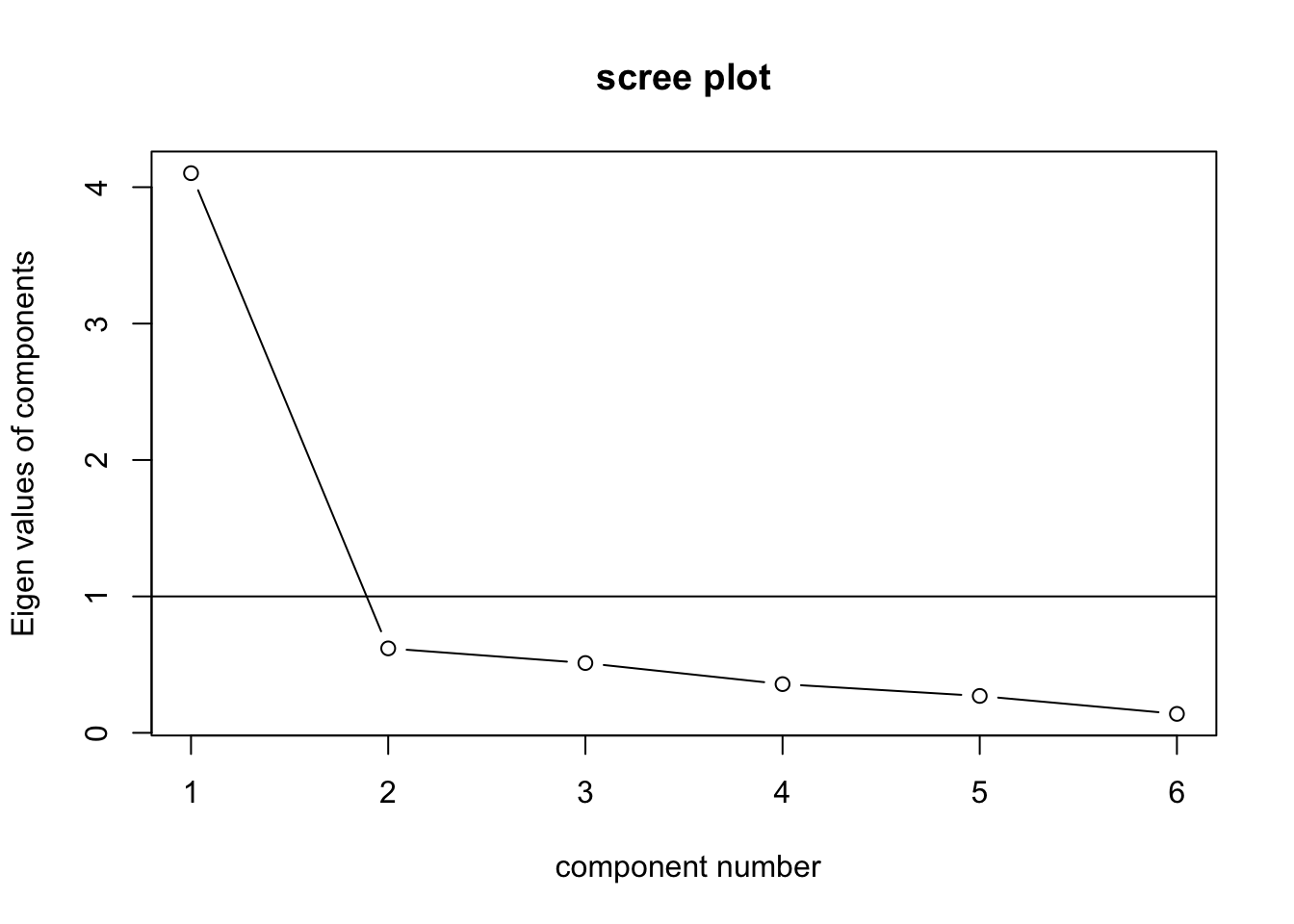
spearman.pc$loadings##
## Loadings:
## PC1 PC2 PC3 PC4 PC5 PC6
## XC 0.937 -0.139 -0.311
## XF 0.894 0.136 -0.381 0.167
## XE 0.842 -0.245 -0.457 0.111
## XM 0.804 0.200 -0.399 0.339 0.198
## XP 0.743 -0.560 0.277 0.221
## XT 0.721 0.506 0.464
##
## PC1 PC2 PC3 PC4 PC5 PC6
## SS loadings 4.103 0.619 0.512 0.357 0.270 0.139
## Proportion Var 0.684 0.103 0.085 0.060 0.045 0.023
## Cumulative Var 0.684 0.787 0.872 0.932 0.977 1.0003. Run PAF with the data
Here you can use the fa() function in the existing R
package psych. You need to specify fm='pa' to
implement PAF. Specify SMC=TRUE as we want to use squared
multiple correlations \(R^2\) instead
of 1 as initial communality estimate (the diagonal elements).
(spearman.pa1 <- fa(spearman,n.obs = 22, rotate = 'none', fm = 'pa', nfactors = 1, SMC = T)) # extract one factor## Factor Analysis using method = pa
## Call: fa(r = spearman, nfactors = 1, n.obs = 22, rotate = "none", SMC = T,
## fm = "pa")
## Standardized loadings (pattern matrix) based upon correlation matrix
## PA1 h2 u2 com
## XC 0.96 0.92 0.084 1
## XF 0.88 0.78 0.222 1
## XE 0.80 0.64 0.355 1
## XM 0.75 0.56 0.437 1
## XP 0.67 0.45 0.547 1
## XT 0.65 0.42 0.583 1
##
## PA1
## SS loadings 3.77
## Proportion Var 0.63
##
## Mean item complexity = 1
## Test of the hypothesis that 1 factor is sufficient.
##
## The degrees of freedom for the null model are 15 and the objective function was 4.05 with Chi Square of 73.56
## The degrees of freedom for the model are 9 and the objective function was 0.09
##
## The root mean square of the residuals (RMSR) is 0.03
## The df corrected root mean square of the residuals is 0.04
##
## The harmonic number of observations is 22 with the empirical chi square 0.53 with prob < 1
## The total number of observations was 22 with Likelihood Chi Square = 1.63 with prob < 1
##
## Tucker Lewis Index of factoring reliability = 1.22
## RMSEA index = 0 and the 90 % confidence intervals are 0 0
## BIC = -26.19
## Fit based upon off diagonal values = 1
## Measures of factor score adequacy
## PA1
## Correlation of (regression) scores with factors 0.98
## Multiple R square of scores with factors 0.95
## Minimum correlation of possible factor scores 0.90spearman.pa1$communality## XC XF XE XM XP XT
## 0.9157796 0.7779349 0.6446360 0.5627324 0.4534621 0.4173629spearman.pa1$Vaccounted## PA1
## SS loadings 3.7719079
## Proportion Var 0.6286513spearman.pa1$loadings##
## Loadings:
## PA1
## XC 0.957
## XF 0.882
## XE 0.803
## XM 0.750
## XP 0.673
## XT 0.646
##
## PA1
## SS loadings 3.772
## Proportion Var 0.629We can see that PCA in general overestimates the factor loadings, compared to PAF.
##          PCA       PAF
## XC 0.9365266 0.9569637
## XF 0.8939569 0.8820062
## XE 0.8420386 0.8028923
## XM 0.8041646 0.7501549
## XP 0.7425730 0.6733959
## XT 0.7206978 0.6460363
PAF Example 2: Analyzing Hotelling’s data using PAF
1. Prepare data
Here are have a correlation matrix obtained in a sample of 200 seventh grade students on tests of 1) reading speed, 2) reading power, 3) arithmetic speed, and 4) arithmetic power.
hotelling## readspd readpwr arithspd arithpwr
## readspd 1.000 0.698 0.264 0.081
## readpwr 0.698 1.000 -0.061 0.092
## arithspd 0.264 -0.061 1.000 0.594
## arithpwr 0.081 0.092 0.594 1.0002. Run PCA to determine the number of factors to extract
(hotelling.pc <- principal(hotelling, nfactors = 4, rotate = 'none'))## Principal Components Analysis
## Call: principal(r = hotelling, nfactors = 4, rotate = "none")
## Standardized loadings (pattern matrix) based upon correlation matrix
## PC1 PC2 PC3 PC4 h2 u2 com
## readspd 0.81 -0.44 -0.29 -0.24 1 -2.2e-16 2.1
## readpwr 0.69 -0.62 0.29 0.23 1 -8.9e-16 2.6
## arithspd 0.61 0.67 -0.38 0.19 1 4.4e-16 2.8
## arithpwr 0.58 0.66 0.46 -0.14 1 -8.9e-16 2.9
##
## PC1 PC2 PC3 PC4
## SS loadings 1.85 1.46 0.52 0.17
## Proportion Var 0.46 0.37 0.13 0.04
## Cumulative Var 0.46 0.83 0.96 1.00
## Proportion Explained 0.46 0.37 0.13 0.04
## Cumulative Proportion 0.46 0.83 0.96 1.00
##
## Mean item complexity = 2.6
## Test of the hypothesis that 4 components are sufficient.
##
## The root mean square of the residuals (RMSR) is 0
##
## Fit based upon off diagonal values = 1VSS.scree(hotelling)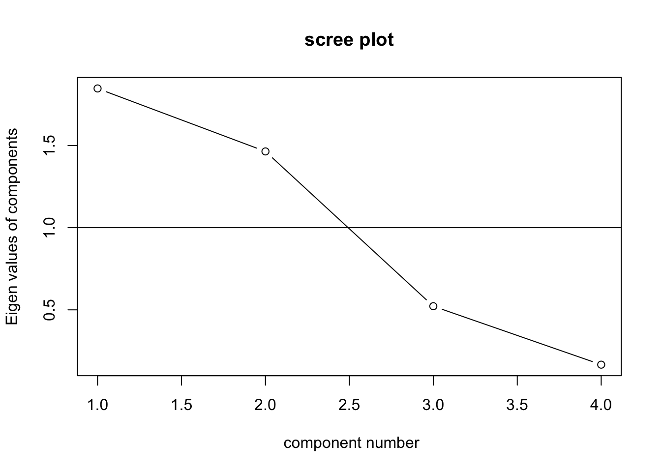
3. Run PAF for factor analysis
You cannnot extract as many number of factors as the number of variables using PAF. Therefore, in this case the maximum number of factors to extract is 3. But based on PCA results, we decide to only extract 2 factors.
Heywood case was detected, indicating we may have negative uniqueness. Therefore, we reduce the number of iterations to see if we can make the Heywood case go away.
(hotelling.pa3 <- fa(hotelling, n.obs = 200, nfactors = 3, rotate = 'none', fm = 'pa', SMC = T))## Factor Analysis using method = pa
## Call: fa(r = hotelling, nfactors = 3, n.obs = 200, rotate = "none",
## SMC = T, fm = "pa")
## Standardized loadings (pattern matrix) based upon correlation matrix
## PA1 PA2 PA3 h2 u2 com
## readspd 0.85 -0.31 -0.28 0.89 0.11 1.5
## readpwr 0.72 -0.51 0.27 0.86 0.14 2.1
## arithspd 0.51 0.73 -0.21 0.84 0.16 2.0
## arithpwr 0.43 0.61 0.34 0.67 0.33 2.4
##
## PA1 PA2 PA3
## SS loadings 1.69 1.26 0.31
## Proportion Var 0.42 0.32 0.08
## Cumulative Var 0.42 0.74 0.82
## Proportion Explained 0.52 0.39 0.09
## Cumulative Proportion 0.52 0.91 1.00
##
## Mean item complexity = 2
## Test of the hypothesis that 3 factors are sufficient.
##
## The degrees of freedom for the null model are 6 and the objective function was 1.45 with Chi Square of 285.14
## The degrees of freedom for the model are -3 and the objective function was 0
##
## The root mean square of the residuals (RMSR) is 0
## The df corrected root mean square of the residuals is NA
##
## The harmonic number of observations is 200 with the empirical chi square 0 with prob < NA
## The total number of observations was 200 with Likelihood Chi Square = 0 with prob < NA
##
## Tucker Lewis Index of factoring reliability = 1.022
## Fit based upon off diagonal values = 1
## Measures of factor score adequacy
## PA1 PA2 PA3
## Correlation of (regression) scores with factors 0.96 0.93 0.79
## Multiple R square of scores with factors 0.92 0.87 0.63
## Minimum correlation of possible factor scores 0.84 0.74 0.26(hotelling.pa2 <- fa(hotelling, n.obs = 200, nfactors = 2, rotate = 'none', fm = 'pa', SMC = T)) ## maximum iteration exceeded## Warning in fa.stats(r = r, f = f, phi = phi, n.obs = n.obs, np.obs = np.obs, :
## The estimated weights for the factor scores are probably incorrect. Try a
## different factor score estimation method.## Warning in fac(r = r, nfactors = nfactors, n.obs = n.obs, rotate = rotate, : An
## ultra-Heywood case was detected. Examine the results carefully## Factor Analysis using method = pa
## Call: fa(r = hotelling, nfactors = 2, n.obs = 200, rotate = "none",
## SMC = T, fm = "pa")
## Standardized loadings (pattern matrix) based upon correlation matrix
## PA1 PA2 h2 u2 com
## readspd 0.49 0.60 0.60 0.40 1.9
## readpwr 0.36 0.87 0.89 0.11 1.3
## arithspd 1.09 -0.49 1.43 -0.43 1.4
## arithpwr 0.47 -0.14 0.24 0.76 1.2
##
## PA1 PA2
## SS loadings 1.78 1.38
## Proportion Var 0.44 0.35
## Cumulative Var 0.44 0.79
## Proportion Explained 0.56 0.44
## Cumulative Proportion 0.56 1.00
##
## Mean item complexity = 1.5
## Test of the hypothesis that 2 factors are sufficient.
##
## The degrees of freedom for the null model are 6 and the objective function was 1.45 with Chi Square of 285.14
## The degrees of freedom for the model are -1 and the objective function was 0.08
##
## The root mean square of the residuals (RMSR) is 0.04
## The df corrected root mean square of the residuals is NA
##
## The harmonic number of observations is 200 with the empirical chi square 3.05 with prob < NA
## The total number of observations was 200 with Likelihood Chi Square = 16.23 with prob < NA
##
## Tucker Lewis Index of factoring reliability = 1.373
## Fit based upon off diagonal values = 0.99hotelling.pa2$uniquenesses## readspd readpwr arithspd arithpwr
## 0.4025256 0.1124124 -0.4304365 0.7587586(hotelling.pa2.it16 <- fa(hotelling, n.obs = 200, nfactors = 2, rotate = 'none', fm = 'pa', SMC = T, max.iter = 16))## maximum iteration exceeded## Factor Analysis using method = pa
## Call: fa(r = hotelling, nfactors = 2, n.obs = 200, rotate = "none",
## SMC = T, max.iter = 16, fm = "pa")
## Standardized loadings (pattern matrix) based upon correlation matrix
## PA1 PA2 h2 u2 com
## readspd 0.75 -0.39 0.71 0.288 1.5
## readpwr 0.62 -0.60 0.74 0.257 2.0
## arithspd 0.67 0.73 0.98 0.016 2.0
## arithpwr 0.42 0.41 0.34 0.658 2.0
##
## PA1 PA2
## SS loadings 1.58 1.21
## Proportion Var 0.39 0.30
## Cumulative Var 0.39 0.70
## Proportion Explained 0.57 0.43
## Cumulative Proportion 0.57 1.00
##
## Mean item complexity = 1.9
## Test of the hypothesis that 2 factors are sufficient.
##
## The degrees of freedom for the null model are 6 and the objective function was 1.45 with Chi Square of 285.14
## The degrees of freedom for the model are -1 and the objective function was 0.16
##
## The root mean square of the residuals (RMSR) is 0.05
## The df corrected root mean square of the residuals is NA
##
## The harmonic number of observations is 200 with the empirical chi square 6.07 with prob < NA
## The total number of observations was 200 with Likelihood Chi Square = 30.93 with prob < NA
##
## Tucker Lewis Index of factoring reliability = 1.691
## Fit based upon off diagonal values = 0.98
## Measures of factor score adequacy
## PA1 PA2
## Correlation of (regression) scores with factors 0.96 0.96
## Multiple R square of scores with factors 0.91 0.92
## Minimum correlation of possible factor scores 0.83 0.85You could do rotation with PAF as well.
#oblimin rotation
(hotelling.pa2.ob <- fa(hotelling, n.obs = 200, nfactors = 2, rotate = 'oblimin', fm = 'pa', SMC = T, max.iter = 16, normalize = T))
## maximum iteration exceeded## Loading required namespace: GPArotation## Factor Analysis using method = pa
## Call: fa(r = hotelling, nfactors = 2, n.obs = 200, rotate = "oblimin",
## SMC = T, max.iter = 16, fm = "pa", normalize = T)
## Standardized loadings (pattern matrix) based upon correlation matrix
## PA1 PA2 h2 u2 com
## readspd 0.82 0.13 0.71 0.288 1.1
## readpwr 0.87 -0.11 0.74 0.257 1.0
## arithspd -0.03 1.00 0.98 0.016 1.0
## arithpwr 0.02 0.58 0.34 0.658 1.0
##
## PA1 PA2
## SS loadings 1.42 1.36
## Proportion Var 0.36 0.34
## Cumulative Var 0.36 0.70
## Proportion Explained 0.51 0.49
## Cumulative Proportion 0.51 1.00
##
## With factor correlations of
## PA1 PA2
## PA1 1.00 0.14
## PA2 0.14 1.00
##
## Mean item complexity = 1
## Test of the hypothesis that 2 factors are sufficient.
##
## The degrees of freedom for the null model are 6 and the objective function was 1.45 with Chi Square of 285.14
## The degrees of freedom for the model are -1 and the objective function was 0.16
##
## The root mean square of the residuals (RMSR) is 0.05
## The df corrected root mean square of the residuals is NA
##
## The harmonic number of observations is 200 with the empirical chi square 6.07 with prob < NA
## The total number of observations was 200 with Likelihood Chi Square = 30.93 with prob < NA
##
## Tucker Lewis Index of factoring reliability = 1.691
## Fit based upon off diagonal values = 0.98hotelling.pa2.ob$loadings #loadings after rotation##
## Loadings:
## PA1 PA2
## readspd 0.816 0.132
## readpwr 0.870 -0.113
## arithspd 0.995
## arithpwr 0.582
##
## PA1 PA2
## SS loadings 1.423 1.360
## Proportion Var 0.356 0.340
## Cumulative Var 0.356 0.696hotelling.pa2.ob$Structure #correlations##
## Loadings:
## PA1 PA2
## readspd 0.834 0.243
## readpwr 0.854
## arithspd 0.108 0.992
## arithpwr 0.585
##
## PA1 PA2
## SS loadings 1.447 1.385
## Proportion Var 0.362 0.346
## Cumulative Var 0.362 0.708hotelling.pa2.ob$Phi## PA1 PA2
## PA1 1.0000000 0.1366426
## PA2 0.1366426 1.0000000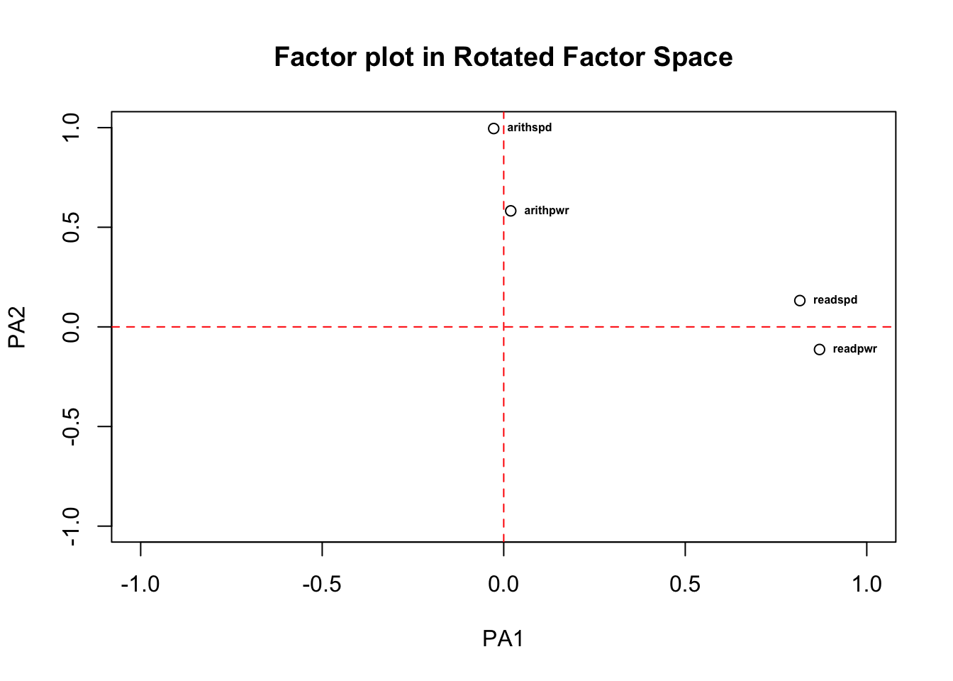
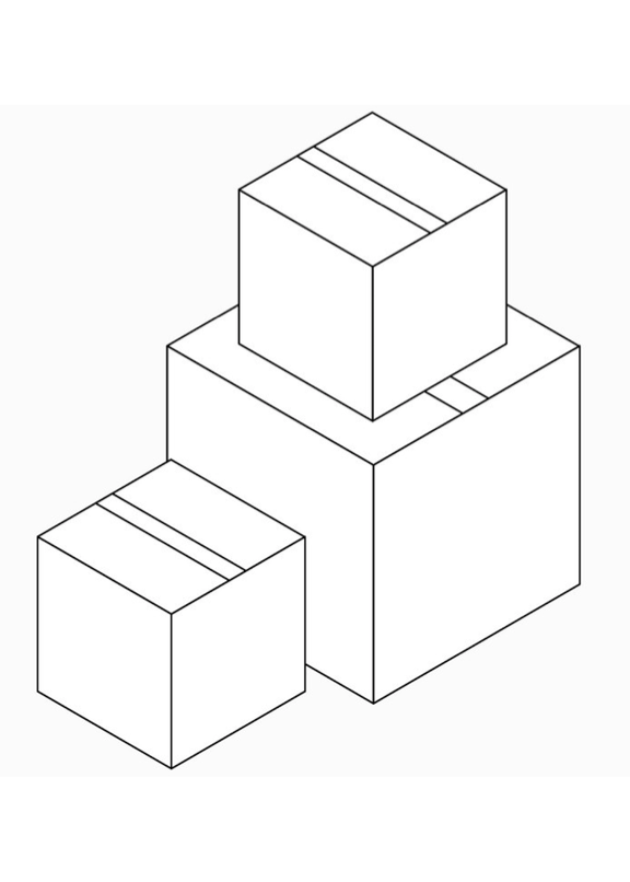
PAF Example 3: Thurstone’s Box Problem
Fourty boxes of varying dimensions are each measured in terms of the ten measures: \(X^2,Y^2,Z^2,XY,XZ,YZ,\text{log}X,\text{log}Y,\text{log}Z,XYZ\), where \(X\) is length, \(Y\) is width, \(Z\) is height.
We know the truth is that there are three “latent factors”: length, width, and height.
1. Prepare data
box.data## Xsq Ysq Zsq XY XZ YZ logX logY logZ XYZ
## Xsq 1.00 0.23 0.08 0.64 0.42 0.15 0.92 0.10 0.10 0.46
## Ysq 0.23 1.00 0.17 0.84 0.21 0.57 0.37 0.93 0.13 0.53
## Zsq 0.08 0.17 1.00 0.14 0.85 0.84 0.16 0.27 0.91 0.77
## XY 0.64 0.84 0.14 1.00 0.34 0.50 0.73 0.76 0.12 0.65
## XZ 0.42 0.21 0.85 0.34 1.00 0.78 0.50 0.22 0.87 0.87
## YZ 0.15 0.57 0.84 0.50 0.78 1.00 0.30 0.64 0.81 0.91
## logX 0.92 0.37 0.16 0.73 0.50 0.30 1.00 0.28 0.18 0.59
## logY 0.10 0.93 0.27 0.76 0.22 0.64 0.28 1.00 0.21 0.58
## logZ 0.10 0.13 0.91 0.12 0.87 0.81 0.18 0.21 1.00 0.76
## XYZ 0.46 0.53 0.77 0.65 0.87 0.91 0.59 0.58 0.76 1.002. PCA
(box.pc <- principal(box.data, nfactors = 10, rotate = 'none'))## Principal Components Analysis
## Call: principal(r = box.data, nfactors = 10, rotate = "none")
## Standardized loadings (pattern matrix) based upon correlation matrix
## PC1 PC2 PC3 PC4 PC5 PC6 PC7 PC8 PC9 PC10 h2 u2 com
## Xsq 0.51 0.47 0.70 0.03 0.13 -0.04 0.08 0.01 0.09 0.00 1 -4.4e-16 2.8
## Ysq 0.65 0.52 -0.51 0.16 0.06 -0.02 -0.06 -0.08 0.01 -0.04 1 7.8e-16 3.1
## Zsq 0.74 -0.62 -0.02 -0.08 0.22 0.00 -0.05 0.02 -0.05 -0.01 1 7.8e-16 2.2
## XY 0.74 0.65 -0.05 0.01 -0.02 -0.11 0.05 0.07 -0.11 0.03 1 -4.4e-16 2.1
## XZ 0.84 -0.40 0.29 0.10 -0.07 -0.05 -0.17 0.04 0.04 0.03 1 1.2e-15 1.9
## YZ 0.91 -0.28 -0.26 -0.09 -0.04 -0.05 0.06 -0.14 0.03 0.04 1 2.6e-15 1.5
## logX 0.64 0.48 0.57 -0.05 -0.04 0.16 -0.06 -0.07 -0.06 0.00 1 -2.9e-15 3.1
## logY 0.67 0.39 -0.61 -0.06 0.02 0.13 0.00 0.09 0.06 0.03 1 2.9e-15 2.8
## logZ 0.73 -0.64 0.04 0.17 -0.04 0.10 0.14 0.02 -0.03 -0.01 1 2.2e-15 2.2
## XYZ 0.97 -0.11 0.04 -0.12 -0.12 -0.06 0.02 0.04 0.03 -0.07 1 1.0e-15 1.1
##
## PC1 PC2 PC3 PC4 PC5 PC6 PC7 PC8 PC9 PC10
## SS loadings 5.62 2.35 1.59 0.10 0.09 0.08 0.07 0.05 0.03 0.01
## Proportion Var 0.56 0.24 0.16 0.01 0.01 0.01 0.01 0.00 0.00 0.00
## Cumulative Var 0.56 0.80 0.96 0.97 0.98 0.98 0.99 1.00 1.00 1.00
## Proportion Explained 0.56 0.24 0.16 0.01 0.01 0.01 0.01 0.00 0.00 0.00
## Cumulative Proportion 0.56 0.80 0.96 0.97 0.98 0.98 0.99 1.00 1.00 1.00
##
## Mean item complexity = 2.3
## Test of the hypothesis that 10 components are sufficient.
##
## The root mean square of the residuals (RMSR) is 0
##
## Fit based upon off diagonal values = 1box.pc$loadings##
## Loadings:
## PC1 PC2 PC3 PC4 PC5 PC6 PC7 PC8 PC9 PC10
## Xsq 0.507 0.473 0.696 0.127
## Ysq 0.653 0.521 -0.511 0.159
## Zsq 0.740 -0.625 0.220
## XY 0.737 0.649 -0.113 -0.109
## XZ 0.839 -0.404 0.287 -0.168
## YZ 0.905 -0.276 -0.258 -0.141
## logX 0.638 0.479 0.568 0.160
## logY 0.666 0.390 -0.608 0.133
## logZ 0.726 -0.641 0.166 0.101 0.141
## XYZ 0.973 -0.109 -0.121 -0.119
##
## PC1 PC2 PC3 PC4 PC5 PC6 PC7 PC8 PC9 PC10
## SS loadings 5.622 2.350 1.594 0.099 0.092 0.077 0.073 0.047 0.035 0.011
## Proportion Var 0.562 0.235 0.159 0.010 0.009 0.008 0.007 0.005 0.003 0.001
## Cumulative Var 0.562 0.797 0.957 0.967 0.976 0.983 0.991 0.995 0.999 1.000VSS.scree(box.data)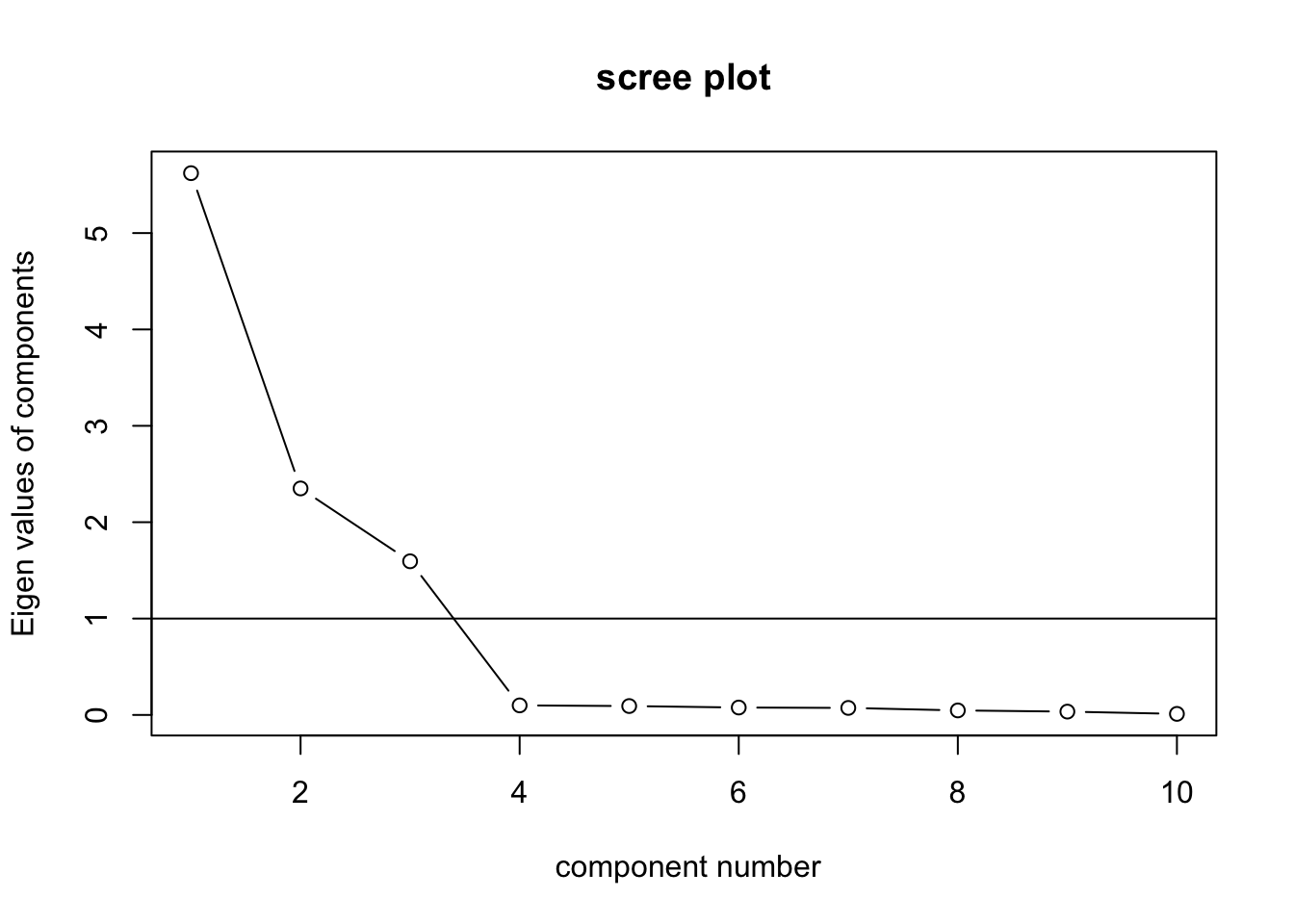
3. PAF
PCA suggests we can proceed with three factors.
(box.pa <- fa(box.data, nfactors = 3, n.obs = 40, rotate = 'none', fm = 'pa', SMC = T))## Factor Analysis using method = pa
## Call: fa(r = box.data, nfactors = 3, n.obs = 40, rotate = "none", SMC = T,
## fm = "pa")
## Standardized loadings (pattern matrix) based upon correlation matrix
## PA1 PA2 PA3 h2 u2 com
## Xsq 0.50 0.46 0.68 0.94 0.063 2.7
## Ysq 0.65 0.51 -0.50 0.93 0.068 2.8
## Zsq 0.73 -0.61 -0.02 0.91 0.090 1.9
## XY 0.74 0.64 -0.05 0.96 0.039 2.0
## XZ 0.83 -0.40 0.28 0.94 0.064 1.7
## YZ 0.90 -0.28 -0.26 0.96 0.041 1.4
## logX 0.63 0.47 0.56 0.93 0.072 2.8
## logY 0.66 0.38 -0.60 0.95 0.055 2.6
## logZ 0.72 -0.63 0.04 0.91 0.089 2.0
## XYZ 0.97 -0.11 0.04 0.96 0.044 1.0
##
## PA1 PA2 PA3
## SS loadings 5.56 2.28 1.53
## Proportion Var 0.56 0.23 0.15
## Cumulative Var 0.56 0.78 0.94
## Proportion Explained 0.59 0.24 0.16
## Cumulative Proportion 0.59 0.84 1.00
##
## Mean item complexity = 2.1
## Test of the hypothesis that 3 factors are sufficient.
##
## The degrees of freedom for the null model are 45 and the objective function was 17.76 with Chi Square of 618.55
## The degrees of freedom for the model are 18 and the objective function was 1.11
##
## The root mean square of the residuals (RMSR) is 0.01
## The df corrected root mean square of the residuals is 0.01
##
## The harmonic number of observations is 40 with the empirical chi square 0.18 with prob < 1
## The total number of observations was 40 with Likelihood Chi Square = 36.28 with prob < 0.0065
##
## Tucker Lewis Index of factoring reliability = 0.915
## RMSEA index = 0.157 and the 90 % confidence intervals are 0.083 0.237
## BIC = -30.12
## Fit based upon off diagonal values = 1
## Measures of factor score adequacy
## PA1 PA2 PA3
## Correlation of (regression) scores with factors 0.99 0.99 0.98
## Multiple R square of scores with factors 0.99 0.97 0.96
## Minimum correlation of possible factor scores 0.98 0.95 0.92You can rotate the solutions as needed. Specify
rotate='varimax to implement Varimax rotation. The
correlations between the variables and factors after rotation clearly
show there are three dimensions: X, Y, and Z
# varimax
(box.pa.var <- fa(box.data, nfactors = 3, n.obs = 40, rotate = 'varimax', fm = 'pa', SMC = T))
## Factor Analysis using method = pa
## Call: fa(r = box.data, nfactors = 3, n.obs = 40, rotate = "varimax",
## SMC = T, fm = "pa")
## Standardized loadings (pattern matrix) based upon correlation matrix
## PA1 PA2 PA3 h2 u2 com
## Xsq 0.08 0.06 0.96 0.94 0.063 1.0
## Ysq 0.11 0.95 0.16 0.93 0.068 1.1
## Zsq 0.95 0.08 -0.02 0.91 0.090 1.0
## XY 0.10 0.77 0.60 0.96 0.039 1.9
## XZ 0.90 0.04 0.36 0.94 0.064 1.3
## YZ 0.84 0.50 0.05 0.96 0.041 1.6
## logX 0.17 0.22 0.92 0.93 0.072 1.2
## logY 0.20 0.95 0.03 0.95 0.055 1.1
## logZ 0.95 0.02 0.02 0.91 0.089 1.0
## XYZ 0.79 0.43 0.39 0.96 0.044 2.1
##
## PA1 PA2 PA3
## SS loadings 4.04 2.89 2.45
## Proportion Var 0.40 0.29 0.24
## Cumulative Var 0.40 0.69 0.94
## Proportion Explained 0.43 0.31 0.26
## Cumulative Proportion 0.43 0.74 1.00
##
## Mean item complexity = 1.3
## Test of the hypothesis that 3 factors are sufficient.
##
## The degrees of freedom for the null model are 45 and the objective function was 17.76 with Chi Square of 618.55
## The degrees of freedom for the model are 18 and the objective function was 1.11
##
## The root mean square of the residuals (RMSR) is 0.01
## The df corrected root mean square of the residuals is 0.01
##
## The harmonic number of observations is 40 with the empirical chi square 0.18 with prob < 1
## The total number of observations was 40 with Likelihood Chi Square = 36.28 with prob < 0.0065
##
## Tucker Lewis Index of factoring reliability = 0.915
## RMSEA index = 0.157 and the 90 % confidence intervals are 0.083 0.237
## BIC = -30.12
## Fit based upon off diagonal values = 1
## Measures of factor score adequacy
## PA1 PA2 PA3
## Correlation of (regression) scores with factors 0.99 0.99 0.98
## Multiple R square of scores with factors 0.98 0.98 0.97
## Minimum correlation of possible factor scores 0.96 0.95 0.94box.pa$loadings##
## Loadings:
## PA1 PA2 PA3
## Xsq 0.504 0.464 0.684
## Ysq 0.650 0.512 -0.497
## Zsq 0.731 -0.612
## XY 0.737 0.645
## XZ 0.834 -0.402 0.282
## YZ 0.903 -0.278 -0.256
## logX 0.633 0.468 0.555
## logY 0.664 0.385 -0.597
## logZ 0.717 -0.628
## XYZ 0.970 -0.112
##
## PA1 PA2 PA3
## SS loadings 5.562 2.282 1.531
## Proportion Var 0.556 0.228 0.153
## Cumulative Var 0.556 0.784 0.938box.pa.var$Structure ##
## Loadings:
## PA1 PA2 PA3
## Xsq 0.962
## Ysq 0.105 0.946 0.162
## Zsq 0.951
## XY 0.769 0.600
## XZ 0.896 0.362
## YZ 0.839 0.502
## logX 0.170 0.220 0.922
## logY 0.198 0.951
## logZ 0.954
## XYZ 0.789 0.428 0.389
##
## PA1 PA2 PA3
## SS loadings 4.039 2.887 2.450
## Proportion Var 0.404 0.289 0.245
## Cumulative Var 0.404 0.693 0.938Specify rotate="oblimin" to implement Oblimin rotation.
Note here that if you ask for the output of “Vaccounted” (variance
accounted for), it is based on the sum of squared loadings (not
correlations).
(box.pa.ob <- fa(box.data, nfactors = 3, n.obs = 40, rotate = 'oblimin', fm = 'pa', SMC = T, normalize = T))## Factor Analysis using method = pa
## Call: fa(r = box.data, nfactors = 3, n.obs = 40, rotate = "oblimin",
## SMC = T, fm = "pa", normalize = T)
## Standardized loadings (pattern matrix) based upon correlation matrix
## PA1 PA2 PA3 h2 u2 com
## Xsq 0.00 -0.08 0.99 0.94 0.063 1.0
## Ysq -0.03 0.96 0.03 0.93 0.068 1.0
## Zsq 0.98 -0.04 -0.11 0.91 0.090 1.0
## XY -0.05 0.72 0.51 0.96 0.039 1.8
## XZ 0.90 -0.12 0.29 0.94 0.064 1.2
## YZ 0.80 0.42 -0.09 0.96 0.041 1.5
## logX 0.07 0.08 0.92 0.93 0.072 1.0
## logY 0.08 0.98 -0.12 0.95 0.055 1.0
## logZ 0.99 -0.10 -0.07 0.91 0.089 1.0
## XYZ 0.73 0.30 0.28 0.96 0.044 1.6
##
## PA1 PA2 PA3
## SS loadings 4.08 2.88 2.42
## Proportion Var 0.41 0.29 0.24
## Cumulative Var 0.41 0.70 0.94
## Proportion Explained 0.43 0.31 0.26
## Cumulative Proportion 0.43 0.74 1.00
##
## With factor correlations of
## PA1 PA2 PA3
## PA1 1.00 0.28 0.22
## PA2 0.28 1.00 0.29
## PA3 0.22 0.29 1.00
##
## Mean item complexity = 1.2
## Test of the hypothesis that 3 factors are sufficient.
##
## The degrees of freedom for the null model are 45 and the objective function was 17.76 with Chi Square of 618.55
## The degrees of freedom for the model are 18 and the objective function was 1.11
##
## The root mean square of the residuals (RMSR) is 0.01
## The df corrected root mean square of the residuals is 0.01
##
## The harmonic number of observations is 40 with the empirical chi square 0.18 with prob < 1
## The total number of observations was 40 with Likelihood Chi Square = 36.28 with prob < 0.0065
##
## Tucker Lewis Index of factoring reliability = 0.915
## RMSEA index = 0.157 and the 90 % confidence intervals are 0.083 0.237
## BIC = -30.12
## Fit based upon off diagonal values = 1
## Measures of factor score adequacy
## PA1 PA2 PA3
## Correlation of (regression) scores with factors 0.99 0.99 0.99
## Multiple R square of scores with factors 0.98 0.98 0.97
## Minimum correlation of possible factor scores 0.97 0.96 0.95box.pa.ob$loadings##
## Loadings:
## PA1 PA2 PA3
## Xsq 0.988
## Ysq 0.965
## Zsq 0.981 -0.112
## XY 0.717 0.512
## XZ 0.897 -0.120 0.291
## YZ 0.802 0.415
## logX 0.918
## logY 0.977 -0.119
## logZ 0.990 -0.103
## XYZ 0.731 0.296 0.276
##
## PA1 PA2 PA3
## SS loadings 3.939 2.700 2.283
## Proportion Var 0.394 0.270 0.228
## Cumulative Var 0.394 0.664 0.892box.pa.ob$Phi## PA1 PA2 PA3
## PA1 1.0000000 0.2830204 0.2173696
## PA2 0.2830204 1.0000000 0.2912642
## PA3 0.2173696 0.2912642 1.0000000box.pa.ob$Vaccounted ## PA1 PA2 PA3
## SS loadings 4.0779286 2.8762902 2.4210434
## Proportion Var 0.4077929 0.2876290 0.2421043
## Cumulative Var 0.4077929 0.6954219 0.9375262
## Proportion Explained 0.4349669 0.3067957 0.2582374
## Cumulative Proportion 0.4349669 0.7417626 1.0000000# SS structure coefficients
(str.coef <- box.pa.ob$Structure)##
## Loadings:
## PA1 PA2 PA3
## Xsq 0.190 0.211 0.965
## Ysq 0.248 0.965 0.304
## Zsq 0.946 0.206
## XY 0.263 0.852 0.710
## XZ 0.926 0.219 0.452
## YZ 0.900 0.616 0.204
## logX 0.292 0.369 0.956
## logY 0.326 0.964 0.182
## logZ 0.945 0.156 0.114
## XYZ 0.875 0.584 0.521
##
## PA1 PA2 PA3
## SS loadings 4.578 3.600 3.014
## Proportion Var 0.458 0.360 0.301
## Cumulative Var 0.458 0.818 1.119colSums(str.coef^2)## PA1 PA2 PA3
## 4.578412 3.600034 3.013889PAF Example 4: An assessment issue
Does the format of items determine the type of skills one can assess? If so, we expect to see two factors that differentiate between the types of items: multiple choices vs. constructed responses.
1. Prepare data
Hancock (1994) constructed all examinations for two educational measurement/statistics classes as half multiple-choice (MC) and half constructed-response (CR), containing equal number of items in each format written for the knowledge (\(know\)), comprehension(\(comp\)),application (\(appl\)), and analysis (\(anal\)) levels of Bloom’s Taxonomy.
test.data## MCknow MCcomp MCappl MCanal CRknow CRcomp CRappl CRanal
## MCknow 1.000 0.410 0.221 0.218 0.513 0.303 0.189 0.359
## MCcomp 0.410 1.000 0.502 0.386 0.270 0.183 0.220 0.465
## MCappl 0.221 0.502 1.000 0.528 0.106 0.107 0.595 0.528
## MCanal 0.218 0.386 0.528 1.000 0.218 0.175 0.556 0.515
## CRknow 0.513 0.270 0.106 0.218 1.000 0.434 0.316 0.266
## CRcomp 0.303 0.183 0.107 0.175 0.434 1.000 0.328 0.244
## CRappl 0.189 0.220 0.595 0.556 0.316 0.328 1.000 0.433
## CRanal 0.359 0.465 0.528 0.515 0.266 0.244 0.433 1.0002. PCA
(test.pc <- principal(test.data, nfactors = 8, rotate = 'none'))## Principal Components Analysis
## Call: principal(r = test.data, nfactors = 8, rotate = "none")
## Standardized loadings (pattern matrix) based upon correlation matrix
## PC1 PC2 PC3 PC4 PC5 PC6 PC7 PC8 h2 u2 com
## MCknow 0.58 0.51 -0.38 -0.24 -0.01 -0.26 0.36 -0.03 1 -4.4e-16 4.4
## MCcomp 0.67 -0.04 -0.55 0.30 0.23 0.27 -0.08 -0.18 1 -6.7e-16 3.3
## MCappl 0.73 -0.48 -0.04 0.05 0.31 -0.22 -0.02 0.31 1 8.9e-16 2.8
## MCanal 0.72 -0.34 0.14 -0.18 -0.24 0.42 0.27 0.08 1 5.6e-16 3.1
## CRknow 0.55 0.64 0.09 -0.32 0.09 0.18 -0.35 0.12 1 1.1e-16 3.5
## CRcomp 0.48 0.53 0.43 0.53 -0.03 0.01 0.13 0.07 1 -1.1e-15 4.1
## CRappl 0.72 -0.22 0.51 -0.17 0.21 -0.14 -0.01 -0.30 1 2.2e-16 2.9
## CRanal 0.76 -0.16 -0.13 0.10 -0.50 -0.23 -0.26 -0.04 1 -4.4e-16 2.5
##
## PC1 PC2 PC3 PC4 PC5 PC6 PC7 PC8
## SS loadings 3.44 1.38 0.95 0.60 0.51 0.47 0.41 0.25
## Proportion Var 0.43 0.17 0.12 0.07 0.06 0.06 0.05 0.03
## Cumulative Var 0.43 0.60 0.72 0.80 0.86 0.92 0.97 1.00
## Proportion Explained 0.43 0.17 0.12 0.07 0.06 0.06 0.05 0.03
## Cumulative Proportion 0.43 0.60 0.72 0.80 0.86 0.92 0.97 1.00
##
## Mean item complexity = 3.3
## Test of the hypothesis that 8 components are sufficient.
##
## The root mean square of the residuals (RMSR) is 0
##
## Fit based upon off diagonal values = 1test.pc$loadings##
## Loadings:
## PC1 PC2 PC3 PC4 PC5 PC6 PC7 PC8
## MCknow 0.583 0.509 -0.383 -0.236 -0.262 0.359
## MCcomp 0.666 -0.551 0.297 0.230 0.268 -0.178
## MCappl 0.727 -0.479 0.306 -0.219 0.308
## MCanal 0.720 -0.344 0.141 -0.178 -0.240 0.421 0.266
## CRknow 0.551 0.642 -0.320 0.180 -0.346 0.119
## CRcomp 0.475 0.534 0.434 0.527 0.134
## CRappl 0.715 -0.217 0.511 -0.169 0.205 -0.136 -0.302
## CRanal 0.756 -0.162 -0.133 0.105 -0.503 -0.230 -0.258
##
## PC1 PC2 PC3 PC4 PC5 PC6 PC7 PC8
## SS loadings 3.443 1.379 0.946 0.598 0.508 0.470 0.411 0.246
## Proportion Var 0.430 0.172 0.118 0.075 0.064 0.059 0.051 0.031
## Cumulative Var 0.430 0.603 0.721 0.796 0.859 0.918 0.969 1.000VSS.scree(test.data) # 2 factors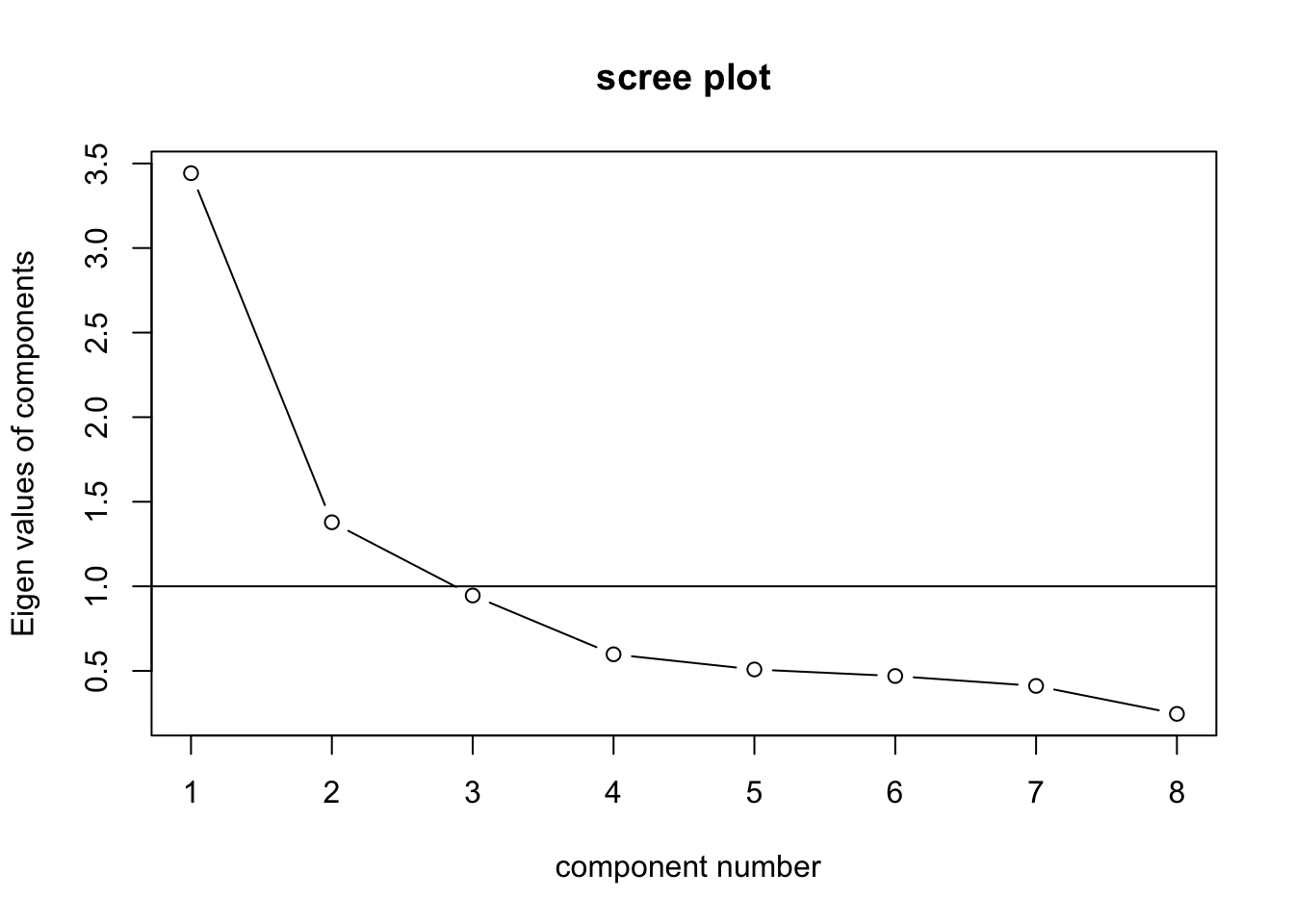
VSS(test.data) #MAP says 1 factor## n.obs was not specified and was arbitrarily set to 1000. This only affects the chi square values.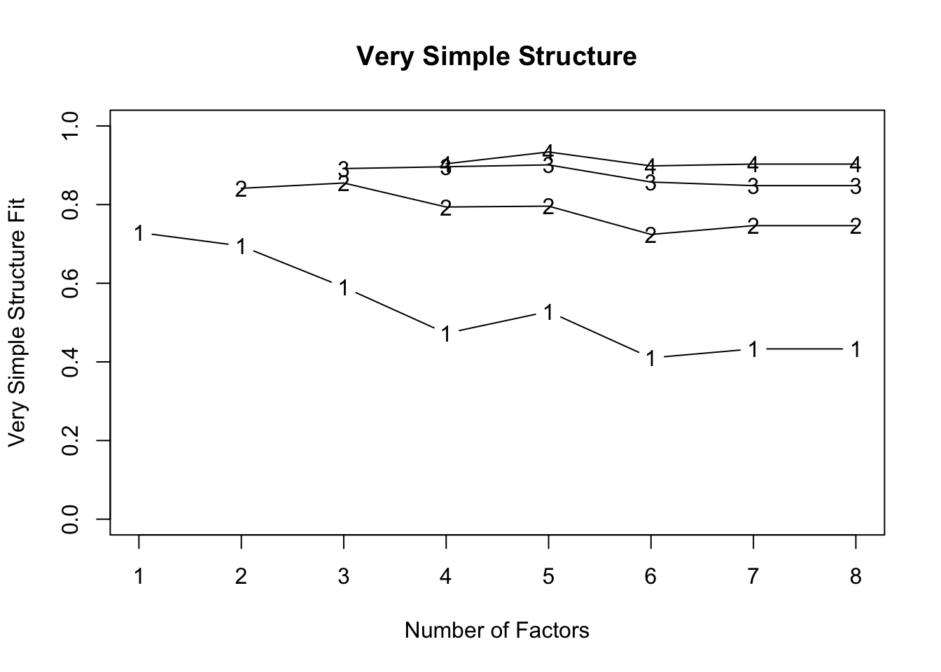
##
## Very Simple Structure
## Call: vss(x = x, n = n, rotate = rotate, diagonal = diagonal, fm = fm,
##     n.obs = n.obs, plot = plot, title = title, use = use, cor = cor)
## VSS complexity 1 achieves a maximimum of 0.73  with  1  factors
## VSS complexity 2 achieves a maximimum of 0.85  with  3  factors
##
## The Velicer MAP achieves a minimum of 0.06  with  1  factors
## BIC achieves a minimum of  -6.63  with  3  factors
## Sample Size adjusted BIC achieves a minimum of  4.87  with  4  factors
##
## Statistics by number of factors
##   vss1 vss2   map dof   chisq     prob sqresid  fit RMSEA   BIC SABIC complex
## 1 0.73 0.00 0.062  20 8.3e+02 5.7e-162    4.26 0.73 0.201 687.3 750.8     1.0
## 2 0.69 0.84 0.068  13 3.5e+02  7.2e-67    2.49 0.84 0.161 260.3 301.6     1.2
## 3 0.59 0.85 0.100   7 4.2e+01  5.9e-07    1.70 0.89 0.070  -6.6  15.6     1.5
## 4 0.47 0.79 0.168   2 1.2e+01  2.1e-03    1.51 0.90 0.072  -1.5   4.9     1.7
## 5 0.53 0.80 0.253  -2 1.6e+00       NA    0.92 0.94    NA    NA    NA     1.6
## 6 0.41 0.72 0.471  -5 2.6e-11       NA    1.12 0.93    NA    NA    NA     2.1
## 7 0.43 0.75 1.000  -7 0.0e+00       NA    1.13 0.93    NA    NA    NA     2.1
## 8 0.43 0.75    NA  -8 0.0e+00       NA    1.13 0.93    NA    NA    NA     2.1
##    eChisq    SRMR eCRMS  eBIC
## 1 8.0e+02 1.2e-01 0.141 657.7
## 2 2.0e+02 6.0e-02 0.088 111.6
## 3 1.6e+01 1.7e-02 0.034 -32.5
## 4 4.9e+00 9.4e-03 0.035  -8.9
## 5 5.4e-01 3.1e-03    NA    NA
## 6 8.5e-12 1.2e-08    NA    NA
## 7 5.6e-16 1.0e-10    NA    NA
## 8 5.6e-16 1.0e-10    NA    NA
3. PAF
(test.pa <- fa(test.data,nfactors = 2, n.obs = 89, rotate = 'none', fm = 'pa', SMC = T)) #no rotation## Factor Analysis using method = pa
## Call: fa(r = test.data, nfactors = 2, n.obs = 89, rotate = "none",
## SMC = T, fm = "pa")
## Standardized loadings (pattern matrix) based upon correlation matrix
## PA1 PA2 h2 u2 com
## MCknow 0.52 0.38 0.42 0.58 1.8
## MCcomp 0.58 -0.02 0.34 0.66 1.0
## MCappl 0.73 -0.45 0.74 0.26 1.7
## MCanal 0.67 -0.23 0.50 0.50 1.2
## CRknow 0.53 0.62 0.66 0.34 2.0
## CRcomp 0.40 0.33 0.27 0.73 1.9
## CRappl 0.65 -0.14 0.45 0.55 1.1
## CRanal 0.70 -0.10 0.50 0.50 1.0
##
## PA1 PA2
## SS loadings 2.95 0.93
## Proportion Var 0.37 0.12
## Cumulative Var 0.37 0.48
## Proportion Explained 0.76 0.24
## Cumulative Proportion 0.76 1.00
##
## Mean item complexity = 1.5
## Test of the hypothesis that 2 factors are sufficient.
##
## The degrees of freedom for the null model are 28 and the objective function was 2.74 with Chi Square of 231.27
## The degrees of freedom for the model are 13 and the objective function was 0.35
##
## The root mean square of the residuals (RMSR) is 0.06
## The df corrected root mean square of the residuals is 0.09
##
## The harmonic number of observations is 89 with the empirical chi square 17.93 with prob < 0.16
## The total number of observations was 89 with Likelihood Chi Square = 29.3 with prob < 0.0059
##
## Tucker Lewis Index of factoring reliability = 0.824
## RMSEA index = 0.118 and the 90 % confidence intervals are 0.061 0.177
## BIC = -29.05
## Fit based upon off diagonal values = 0.97
## Measures of factor score adequacy
## PA1 PA2
## Correlation of (regression) scores with factors 0.93 0.84
## Multiple R square of scores with factors 0.87 0.71
## Minimum correlation of possible factor scores 0.74 0.43(test.pa.ob <- fa(test.data, nfactors = 2, n.obs = 89, rotate = 'oblimin', fm = 'pa', SMC = T, normalize = T)) #oblimin## Factor Analysis using method = pa
## Call: fa(r = test.data, nfactors = 2, n.obs = 89, rotate = "oblimin",
## SMC = T, fm = "pa", normalize = T)
## Standardized loadings (pattern matrix) based upon correlation matrix
## PA1 PA2 h2 u2 com
## MCknow 0.10 0.60 0.42 0.58 1.1
## MCcomp 0.47 0.19 0.34 0.66 1.3
## MCappl 0.93 -0.21 0.74 0.26 1.1
## MCanal 0.71 -0.01 0.50 0.50 1.0
## CRknow -0.08 0.85 0.66 0.34 1.0
## CRcomp 0.04 0.50 0.27 0.73 1.0
## CRappl 0.63 0.09 0.45 0.55 1.0
## CRanal 0.63 0.14 0.50 0.50 1.1
##
## PA1 PA2
## SS loadings 2.42 1.46
## Proportion Var 0.30 0.18
## Cumulative Var 0.30 0.48
## Proportion Explained 0.62 0.38
## Cumulative Proportion 0.62 1.00
##
## With factor correlations of
## PA1 PA2
## PA1 1.00 0.45
## PA2 0.45 1.00
##
## Mean item complexity = 1.1
## Test of the hypothesis that 2 factors are sufficient.
##
## The degrees of freedom for the null model are 28 and the objective function was 2.74 with Chi Square of 231.27
## The degrees of freedom for the model are 13 and the objective function was 0.35
##
## The root mean square of the residuals (RMSR) is 0.06
## The df corrected root mean square of the residuals is 0.09
##
## The harmonic number of observations is 89 with the empirical chi square 17.93 with prob < 0.16
## The total number of observations was 89 with Likelihood Chi Square = 29.3 with prob < 0.0059
##
## Tucker Lewis Index of factoring reliability = 0.824
## RMSEA index = 0.118 and the 90 % confidence intervals are 0.061 0.177
## BIC = -29.05
## Fit based upon off diagonal values = 0.97
## Measures of factor score adequacy
## PA1 PA2
## Correlation of (regression) scores with factors 0.93 0.88
## Multiple R square of scores with factors 0.87 0.78
## Minimum correlation of possible factor scores 0.73 0.56test.pa$loadings##
## Loadings:
## PA1 PA2
## MCknow 0.519 0.383
## MCcomp 0.584
## MCappl 0.731 -0.450
## MCanal 0.667 -0.234
## CRknow 0.531 0.618
## CRcomp 0.402 0.335
## CRappl 0.654 -0.143
## CRanal 0.698 -0.104
##
## PA1 PA2
## SS loadings 2.948 0.930
## Proportion Var 0.369 0.116
## Cumulative Var 0.369 0.485test.pa.ob$loadings##
## Loadings:
## PA1 PA2
## MCknow 0.595
## MCcomp 0.471 0.193
## MCappl 0.933 -0.211
## MCanal 0.710
## CRknow 0.849
## CRcomp 0.501
## CRappl 0.626
## CRanal 0.629 0.144
##
## PA1 PA2
## SS loadings 2.401 1.436
## Proportion Var 0.300 0.180
## Cumulative Var 0.300 0.480test.pa$Structure##
## Loadings:
## PA1 PA2
## MCknow 0.519 0.383
## MCcomp 0.584
## MCappl 0.731 -0.450
## MCanal 0.667 -0.234
## CRknow 0.531 0.618
## CRcomp 0.402 0.335
## CRappl 0.654 -0.143
## CRanal 0.698 -0.104
##
## PA1 PA2
## SS loadings 2.948 0.930
## Proportion Var 0.369 0.116
## Cumulative Var 0.369 0.485test.pa.ob$Structure##
## Loadings:
## PA1 PA2
## MCknow 0.367 0.639
## MCcomp 0.558 0.406
## MCappl 0.838 0.211
## MCanal 0.707 0.315
## CRknow 0.301 0.812
## CRcomp 0.271 0.521
## CRappl 0.665 0.369
## CRanal 0.694 0.428
##
## PA1 PA2
## SS loadings 2.736 1.968
## Proportion Var 0.342 0.246
## Cumulative Var 0.342 0.588test.pa.ob$Phi## PA1 PA2
## PA1 1.0000000 0.4520425
## PA2 0.4520425 1.0000000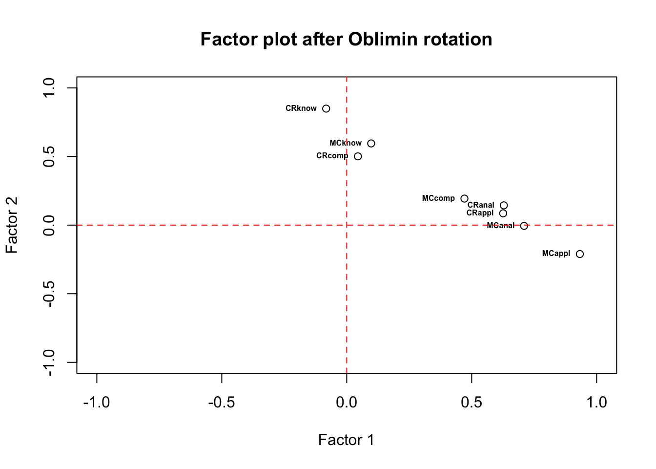
EFA Odds and Ends
Factor Scores
You can obtain the estimated factor scores using different strategies.
PCA scores.
pca_fit <- principal(turtle, scores = T)
head(pca_fit$scores)
## PC1
## [1,] -0.02023085
## [2,] -0.12103463
## [3,] 0.74517897
## [4,] -1.25787459
## [5,] 0.15473068
## [6,] 0.40973895Factor scores via regression.
fa_fit <- fa(turtle, scores = "regression")
head(fa_fit$scores)
## MR1
## [1,] -0.05295795
## [2,] -0.09709426
## [3,] 0.74021981
## [4,] -1.25302724
## [5,] 0.16348607
## [6,] 0.41049973You can try other different factoring methods available within the
fa() function.
Maximum Likelihood
(test.ml <- fa(test.data, nfactors = 2, n.obs=89, rotate = 'none', fm = 'ml', SMC = T))## Factor Analysis using method = ml
## Call: fa(r = test.data, nfactors = 2, n.obs = 89, rotate = "none",
## SMC = T, fm = "ml")
## Standardized loadings (pattern matrix) based upon correlation matrix
## ML1 ML2 h2 u2 com
## MCknow 0.48 0.41 0.40 0.60 1.9
## MCcomp 0.59 -0.01 0.35 0.65 1.0
## MCappl 0.77 -0.39 0.75 0.25 1.5
## MCanal 0.66 -0.15 0.46 0.54 1.1
## CRknow 0.48 0.67 0.69 0.31 1.8
## CRcomp 0.37 0.38 0.28 0.72 2.0
## CRappl 0.69 -0.08 0.48 0.52 1.0
## CRanal 0.69 -0.05 0.47 0.53 1.0
##
## ML1 ML2
## SS loadings 2.93 0.95
## Proportion Var 0.37 0.12
## Cumulative Var 0.37 0.49
## Proportion Explained 0.75 0.25
## Cumulative Proportion 0.75 1.00
##
## Mean item complexity = 1.4
## Test of the hypothesis that 2 factors are sufficient.
##
## The degrees of freedom for the null model are 28 and the objective function was 2.74 with Chi Square of 231.27
## The degrees of freedom for the model are 13 and the objective function was 0.34
##
## The root mean square of the residuals (RMSR) is 0.06
## The df corrected root mean square of the residuals is 0.09
##
## The harmonic number of observations is 89 with the empirical chi square 18.77 with prob < 0.13
## The total number of observations was 89 with Likelihood Chi Square = 28.65 with prob < 0.0073
##
## Tucker Lewis Index of factoring reliability = 0.831
## RMSEA index = 0.116 and the 90 % confidence intervals are 0.058 0.175
## BIC = -29.71
## Fit based upon off diagonal values = 0.97
## Measures of factor score adequacy
## ML1 ML2
## Correlation of (regression) scores with factors 0.93 0.85
## Multiple R square of scores with factors 0.87 0.72
## Minimum correlation of possible factor scores 0.74 0.44Alpha factoring
(test.alpha <- fa(test.data, nfactors = 2, n.obs = 89, rotate = 'none', fm = 'alpha', SMC = T))## Factor Analysis using method = alpha
## Call: fa(r = test.data, nfactors = 2, n.obs = 89, rotate = "none",
## SMC = T, fm = "alpha")
## Standardized loadings (pattern matrix) based upon correlation matrix
## alpha1 alpha2 h2 u2 com
## MCknow 0.55 0.33 0.41 0.59 1.6
## MCcomp 0.56 -0.05 0.32 0.68 1.0
## MCappl 0.71 -0.53 0.78 0.22 1.9
## MCanal 0.66 -0.32 0.53 0.47 1.4
## CRknow 0.58 0.59 0.69 0.31 2.0
## CRcomp 0.42 0.28 0.26 0.74 1.7
## CRappl 0.62 -0.16 0.41 0.59 1.1
## CRanal 0.70 -0.16 0.52 0.48 1.1
##
## alpha1 alpha2
## SS loadings 2.95 0.97
## Proportion Var 0.37 0.12
## Cumulative Var 0.37 0.49
## Proportion Explained 0.75 0.25
## Cumulative Proportion 0.75 1.00
##
## Mean item complexity = 1.5
## Test of the hypothesis that 2 factors are sufficient.
##
## The degrees of freedom for the null model are 28 and the objective function was 2.74 with Chi Square of 231.27
## The degrees of freedom for the model are 13 and the objective function was 0.39
##
## The root mean square of the residuals (RMSR) is 0.06
## The df corrected root mean square of the residuals is 0.09
##
## The harmonic number of observations is 89 with the empirical chi square 18.96 with prob < 0.12
## The total number of observations was 89 with Likelihood Chi Square = 32.07 with prob < 0.0023
##
## Tucker Lewis Index of factoring reliability = 0.794
## RMSEA index = 0.128 and the 90 % confidence intervals are 0.073 0.186
## BIC = -26.29
## Fit based upon off diagonal values = 0.97
## Measures of factor score adequacy
## alpha1 alpha2
## Correlation of (regression) scores with factors 0.94 0.88
## Multiple R square of scores with factors 0.89 0.77
## Minimum correlation of possible factor scores 0.77 0.54The R script for this tutorial can be found here.
© Copyright 2022 Yi Feng and Gregory R. Hancock.