EDMS 657-R Tutorial: Factorial MANOVA and MANOVA for Repeated Measures
Yi Feng & Gregory R. Hancock
University of Maryland, College ParkIn this document we supply two additional examples of MANOVA using R. This document serves as a supplementary material for EDMS 657-Exploratory Latent and Composite Variable Methods, taught by Dr. Gregory R. Hancock at University of Maryland.
Before we get started, let’s make sure we install all the packages we need to use in this demo.
install.packages("ggplot2")
install.packages("psych")
install.packages("agricolae")
install.pacakges("car")
install.pakcages("tidyverse")
devtools::install_github("YiFengEDMS/EDMS657Data")
Example 4: Between-subjects factorial MANOVA
Research Context
Researchers are interested in studying the effects of drugs and physical exercise on people’s weight loss and positive attitude. They wish to test both the main effects and interactions effects.
Step 1: Load the data
library(EDMS657Data)
data("MANOVA2way")
Take a look at the data you just read into R
library(tidyverse)
glimpse(MANOVA2way)
## Rows: 24
## Columns: 5
## $ drug <int> 1, 1, 1, 1, 1, 1, 1, 1, 2, 2, 2, 2, 2, 2, 2, 2, 3, 3, 3…
## $ exercise <int> 1, 1, 1, 1, 0, 0, 0, 0, 1, 1, 1, 1, 0, 0, 0, 0, 1, 1, 1…
## $ wtloss <int> 5, 5, 9, 7, 7, 6, 9, 8, 7, 7, 9, 6, 10, 8, 7, 6, 21, 14…
## $ posattit <int> 6, 4, 9, 6, 10, 6, 7, 10, 6, 7, 12, 8, 13, 7, 6, 9, 15,…
## $ group <fct> "drug A, exercise", "drug A, exercise", "drug A, exerci…#View(MANOVA2way)
str(MANOVA2way)## 'data.frame': 24 obs. of 5 variables:
## $ drug : int 1 1 1 1 1 1 1 1 2 2 ...
## $ exercise: int 1 1 1 1 0 0 0 0 1 1 ...
## $ wtloss : int 5 5 9 7 7 6 9 8 7 7 ...
## $ posattit: int 6 4 9 6 10 6 7 10 6 7 ...
## $ group : Factor w/ 6 levels "drug A, exercise",..: 1 1 1 1 2 2 2 2 3 3 ...head(MANOVA2way)## drug exercise wtloss posattit group
## 1 1 1 5 6 drug A, exercise
## 2 1 1 5 4 drug A, exercise
## 3 1 1 9 9 drug A, exercise
## 4 1 1 7 6 drug A, exercise
## 5 1 0 7 10 drug A, no exercise
## 6 1 0 6 6 drug A, no exerciseNote that “drug” and “exercise” should both be categorical variables.
MANOVA2way <- MANOVA2way %>%
  mutate(drug = factor(drug, labels = c("drug A","drug B","drug C")),
         exercise = factor(exercise, labels = c("no","yes")))
Step 2: Explore the data with descriptive statistics and plots
Descriptive statistics
summary(MANOVA2way)## drug exercise wtloss posattit
## drug A:8 no :12 Min. : 5.00 Min. : 4.000
## drug B:8 yes:12 1st Qu.: 7.00 1st Qu.: 6.000
## drug C:8 Median : 8.50 Median : 8.500
## Mean : 9.75 Mean : 8.667
## 3rd Qu.:12.50 3rd Qu.:10.250
## Max. :21.00 Max. :15.000
## group
## drug A, exercise :4
## drug A, no exercise:4
## drug B, exercise :4
## drug B, no exercise:4
## drug C, exercise :4
## drug C, no exercise:4table(MANOVA2way$drug, MANOVA2way$exercise)##
## no yes
## drug A 4 4
## drug B 4 4
## drug C 4 4Within-group statistics
MANOVA2way %>%
  group_by(drug, exercise) %>%
  summarize(mean_wtloss = mean(wtloss),
            mean_posattit = mean(posattit),
            var_wtloss = var(wtloss),
            var_posattit = var(posattit))
## # A tibble: 6 × 6
## # Groups: drug [3]
## drug exercise mean_wtloss mean_posattit var_wtloss var_posattit
## <fct> <fct> <dbl> <dbl> <dbl> <dbl>
## 1 drug A no 7.5 8.25 1.67 4.25
## 2 drug A yes 6.5 6.25 3.67 4.25
## 3 drug B no 7.75 8.75 2.92 9.58
## 4 drug B yes 7.25 8.25 1.58 6.92
## 5 drug C no 13.5 8.5 6.33 8.33
## 6 drug C yes 16 12 15.3 4.67Descriptive plots
You could visualize the data in whichever way that can better help you understand the data. In this case one possible plot that may be helpful is to draw the group centroids (without showing the indivisual data points).
library(ggplot2)

# The plot is colored by the group
scatterPlot <- ggplot(MANOVA2way, aes(wtloss, posattit, color = drug, shape = exercise),
                      group = interaction(drug, exercise)) +
  geom_point()
scatterPlot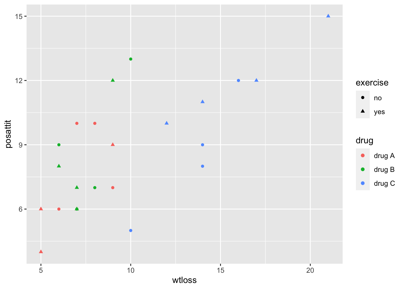
centroids <- aggregate(cbind(wtloss = wtloss, posattit = posattit) ~ drug*exercise, data = MANOVA2way, mean)
centroids$group <- paste0(centroids$drug, ", ", centroids$exercise)

ggplot(centroids, mapping = aes(x = wtloss, y = posattit, color = group, shape = group))+
  geom_point(size=5) +
  ggtitle("Group Centroids") +
  scale_colour_manual(name = "Group",
                      labels = c("drug A, no exercise", "drug B, no exercise",  "drug C, no exercise",  "drug A,  exercise", "drug B,  exercise", "drug C,  exercise"),
                      values = c('#999999','#E69F00',"#56B4E9",'#999999','#E69F00',"#56B4E9")) +
  scale_shape_manual(name = "Group",
                     labels = c("drug A, no exercise", "drug B, no exercise",  "drug C, no exercise",  "drug A,  exercise", "drug B,  exercise", "drug C,  exercise"),
                     values = c(19, 19, 19,17, 17,17)) +
 theme(plot.title = element_text(hjust = 0.5))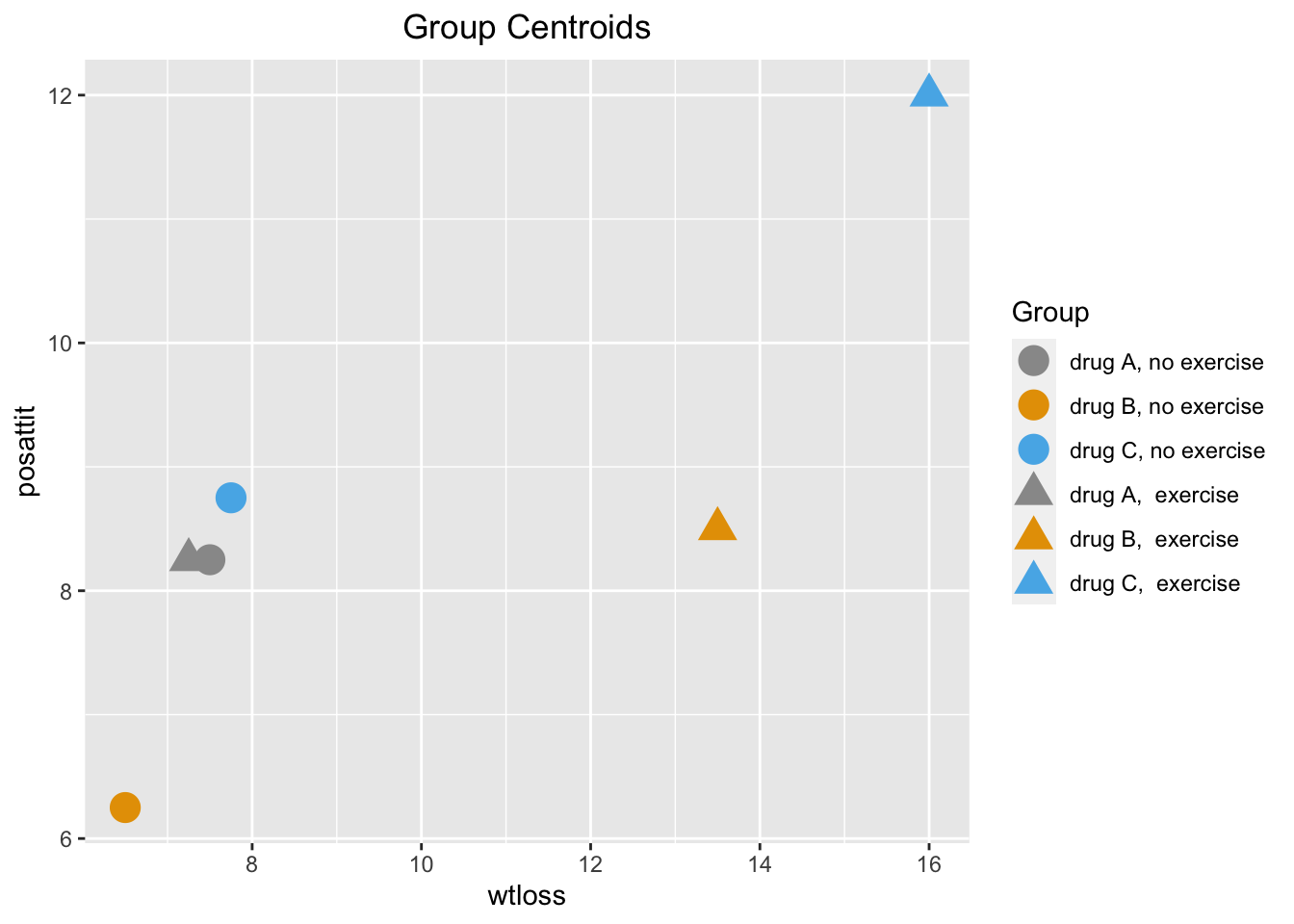
Step 3: Factorial MANOVA Tests
Indicate in the formula that you wish to test the interaction effect between drug and exercise.
manova.model4 <- manova(cbind(wtloss, posattit) ~ drug*exercise, MANOVA2way)
summary(manova.model4)
## Df Pillai approx F num Df den Df Pr(>F)
## drug 2 0.88038 7.0769 4 36 0.0002602 ***
## exercise 1 0.00746 0.0639 2 17 0.9383109
## drug:exercise 2 0.22695 1.1520 4 36 0.3480795
## Residuals 18
## ---
## Signif. codes: 0 '***' 0.001 '**' 0.01 '*' 0.05 '.' 0.1 ' ' 1Step 4: Follow-up Univariate ANOVA
Because the drug main effect is significant, we can proceed with univariate ANOVA to test the effect of drug on each of the outcomes.
aov.wt <- aov(wtloss~drug*exercise, MANOVA2way)
aov.at <- aov(posattit~drug*exercise, MANOVA2way)
We can follow up the significant univariate main effect with Fisher’s LSD test.
(agricolae::LSD.test(aov.wt, "drug"))$groups## wtloss groups
## drug C 14.75 a
## drug B 7.50 b
## drug A 7.00 b(agricolae::LSD.test(aov.at, "drug"))$groups## posattit groups
## drug C 10.25 a
## drug B 8.50 ab
## drug A 7.25 bExample 5: MANOVA for repeated measures
Research Context
Researchers are interested in studying whether the brand of sneakers affects how high individuals can jump up from the ground. A group of subjects were tested repeatedly wearing three different brands of sneakers: Reebok, Nike, and Converse.
Step 1: Load the data
library(EDMS657Data)
data("MANOVA_RM")
Take a look at the data you just read into R
library(tidyverse)
#View(MANOVA_RM)
glimpse(MANOVA_RM)
## Rows: 5
## Columns: 4
## $ id <int> 1, 2, 3, 4, 5
## $ reebok <int> 36, 32, 34, 38, 40
## $ nike <int> 48, 46, 40, 44, 42
## $ converse <int> 36, 38, 34, 40, 42str(MANOVA_RM)## 'data.frame': 5 obs. of 4 variables:
## $ id : int 1 2 3 4 5
## $ reebok : int 36 32 34 38 40
## $ nike : int 48 46 40 44 42
## $ converse: int 36 38 34 40 42head(MANOVA_RM)## id reebok nike converse
## 1 1 36 48 36
## 2 2 32 46 38
## 3 3 34 40 34
## 4 4 38 44 40
## 5 5 40 42 42Compute the within-subject difference scores
MANOVA_RM <- MANOVA_RM %>%
  mutate(id = factor(id),
         diff1 = reebok - nike,
         diff2 = reebok - converse,
         diff3 = nike - converse)
Step 2: Explore the data
Descriptive statistics
summary(MANOVA_RM)## id reebok nike converse diff1 diff2
## 1:1 Min. :32 Min. :40 Min. :34 Min. :-14 Min. :-6
## 2:1 1st Qu.:34 1st Qu.:42 1st Qu.:36 1st Qu.:-12 1st Qu.:-2
## 3:1 Median :36 Median :44 Median :38 Median : -6 Median :-2
## 4:1 Mean :36 Mean :44 Mean :38 Mean : -8 Mean :-2
## 5:1 3rd Qu.:38 3rd Qu.:46 3rd Qu.:40 3rd Qu.: -6 3rd Qu.: 0
## Max. :40 Max. :48 Max. :42 Max. : -2 Max. : 0
## diff3
## Min. : 0
## 1st Qu.: 4
## Median : 6
## Mean : 6
## 3rd Qu.: 8
## Max. :12Descriptive plots
You can do a scatterplot of the individual difference scores along with the single group’s centroid in a two-dimensional space. The third difference score is not needed as it is perfectly multicollinear with the other two difference scores.
scatterPlot5 <- ggplot(MANOVA_RM,aes(diff1, diff2)) + geom_point()+
  xlim(-20,20)+ylim(-20,20)
scatterPlot5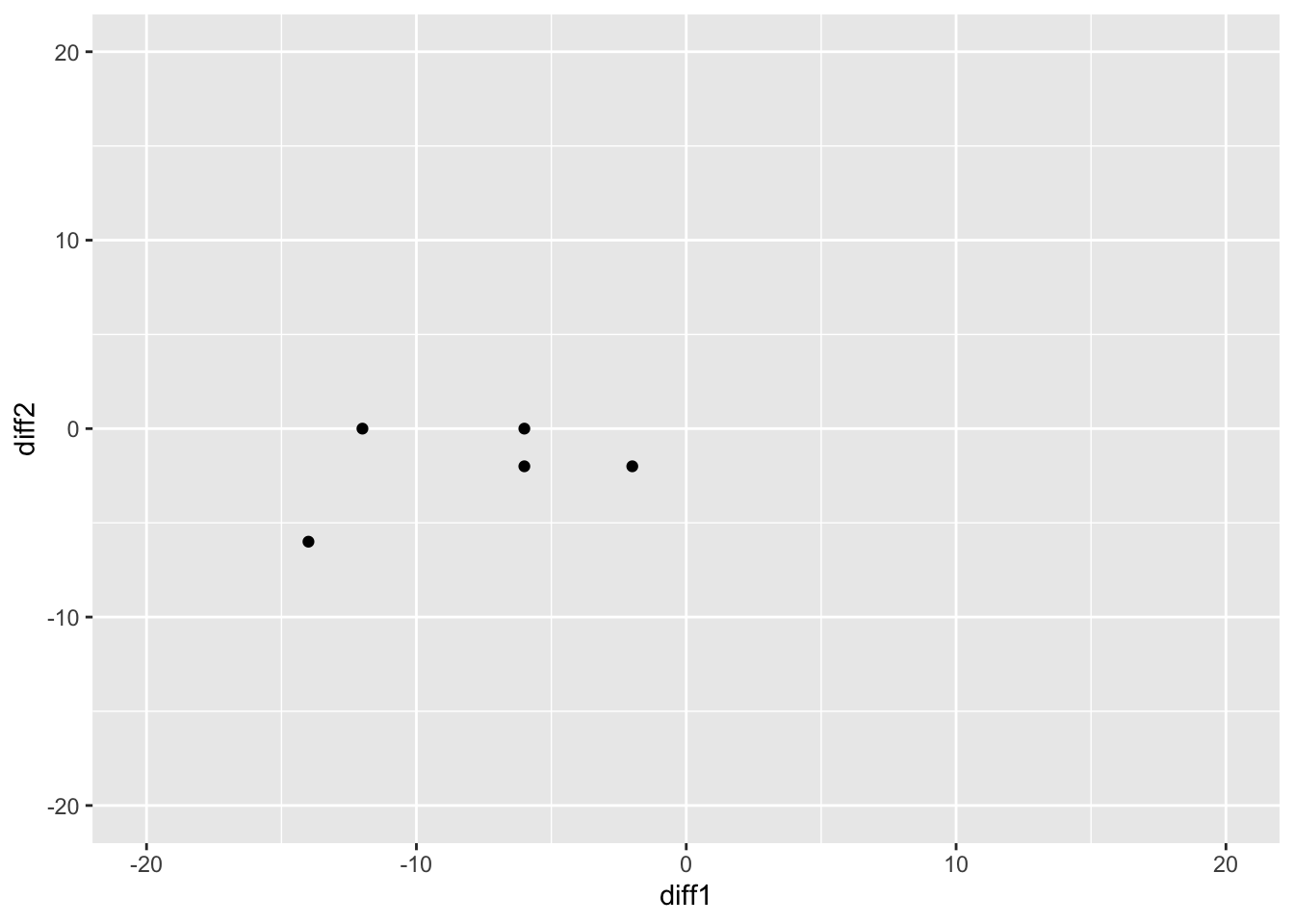
meandiff <- colMeans(MANOVA_RM[,-1])[c("diff1","diff2")]

scatterPlot5 + geom_point(as.data.frame(t(meandiff)),mapping=aes(x=diff1,y=diff2),size=5,shape=17,color="red")+geom_vline(xintercept = 0)+geom_hline(yintercept = 5)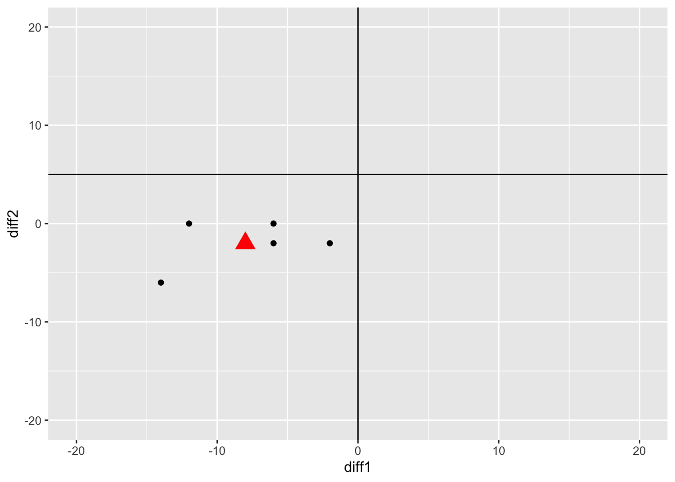
Step 3: Tests using MANOVA for Repeated Measures
We can make use of the Anova(mod, idata, idesign)
function available in the car package to analyze the
repeated measures data. This function is capable of both the univariate
approach (repeated measures ANOVA) and the multivariate approach
(MANOVA).
To use this function, you will need to first create a data frame containing the within-subject factor(s).
manova.model5 <- lm(cbind(reebok, nike, converse) ~ 1, data = MANOVA_RM)

shoes <- as.factor(c(1,2,3))
levels(shoes) <- c("reebok","nike","converse")
shoes.data <- data.frame(shoes)

rm_manova <- car::Anova(manova.model5, idata = shoes.data, idesign = ~shoes)
(summary(rm_manova))$multivariate.tests$shoes
##
## Response transformation matrix:
## shoes1 shoes2
## reebok 1 0
## nike 0 1
## converse -1 -1
##
## Sum of squares and products for the hypothesis:
## shoes1 shoes2
## shoes1 20 -60
## shoes2 -60 180
##
## Sum of squares and products for error:
## shoes1 shoes2
## shoes1 24 4
## shoes2 4 80
##
## Multivariate Tests: shoes
## Df test stat approx F num Df den Df Pr(>F)
## Pillai 1 0.770713 5.042017 2 3 0.10979
## Wilks 1 0.229287 5.042017 2 3 0.10979
## Hotelling-Lawley 1 3.361345 5.042017 2 3 0.10979
## Roy 1 3.361345 5.042017 2 3 0.10979© Copyright 2022 Yi Feng and Gregory R. Hancock.