EDMS 657-R Tutorial: Cluster Analysis
Yi Feng & Gregory R. Hancock
University of Maryland, College ParkIn this document we will discuss how to conduct cluster analysis using R. This document serves as a supplementary material for EDMS 657-Exploratory Latent and Composite Variable Methods, taught by Dr. Gregory R. Hancock at University of Maryland.
install.packages("psych")
install.packages("distances")
install.packages("factoextra")
install.packages("stats")
library(psych)
library(EDMS657Data)Example 1: Hierarchical Cluster Analysis
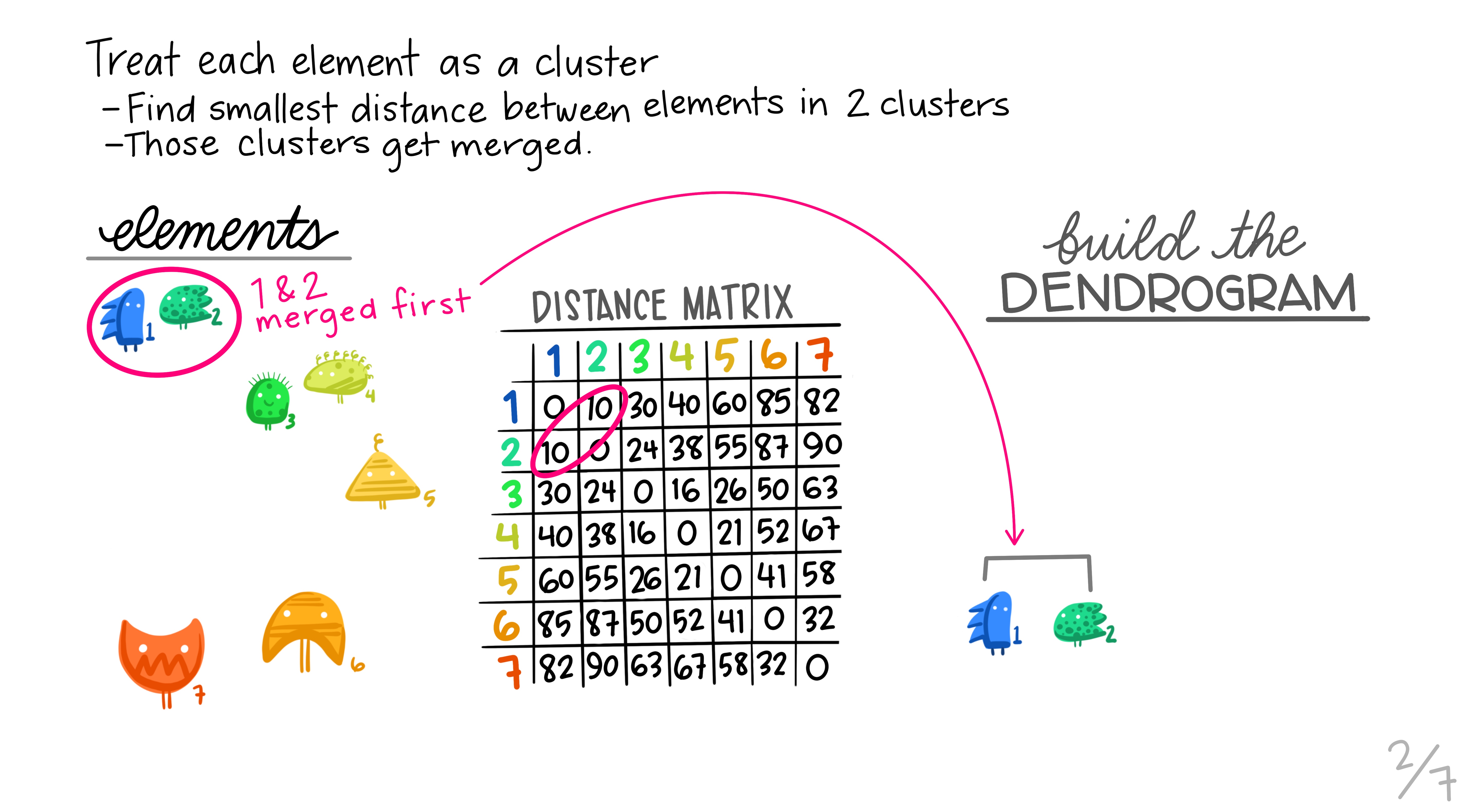
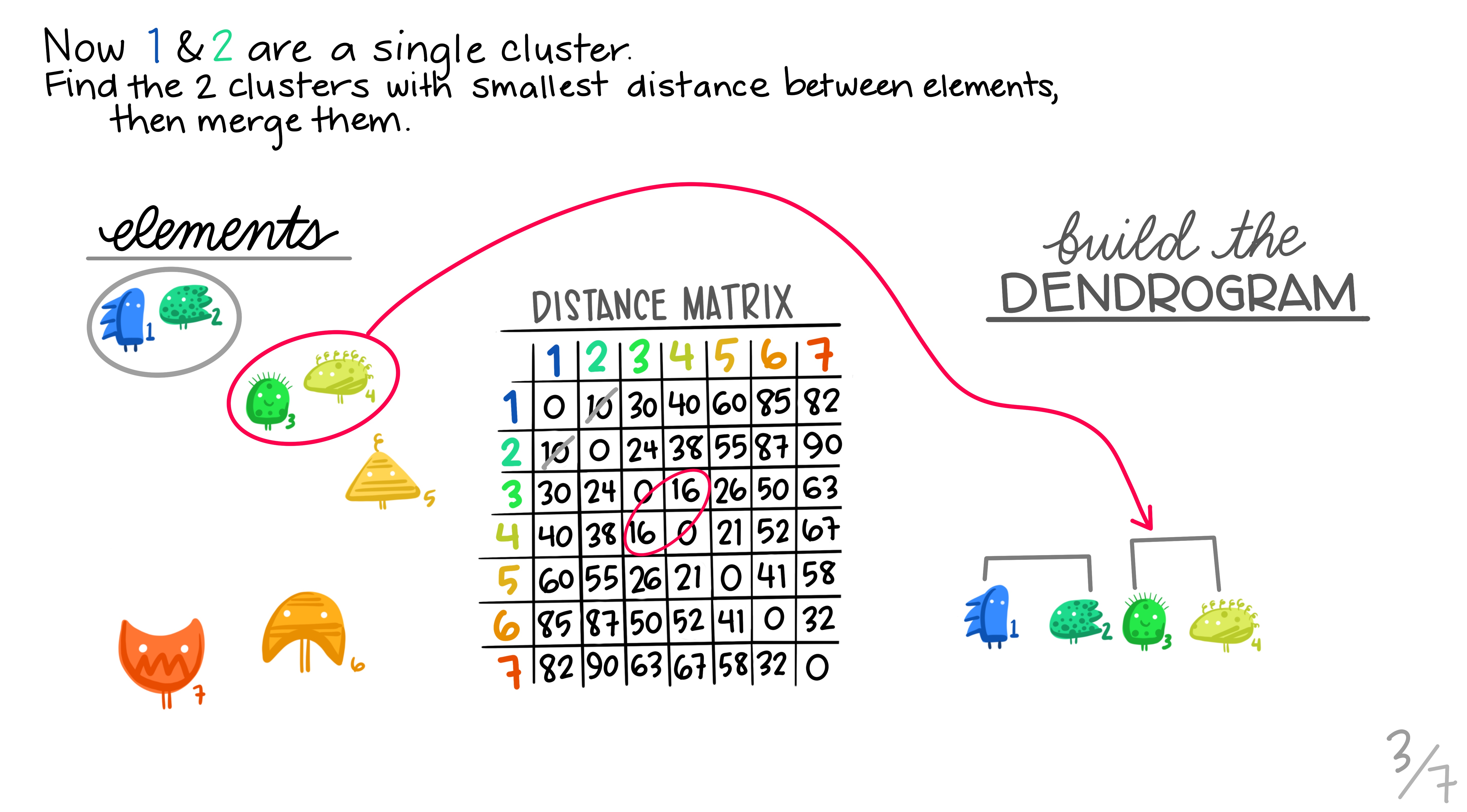
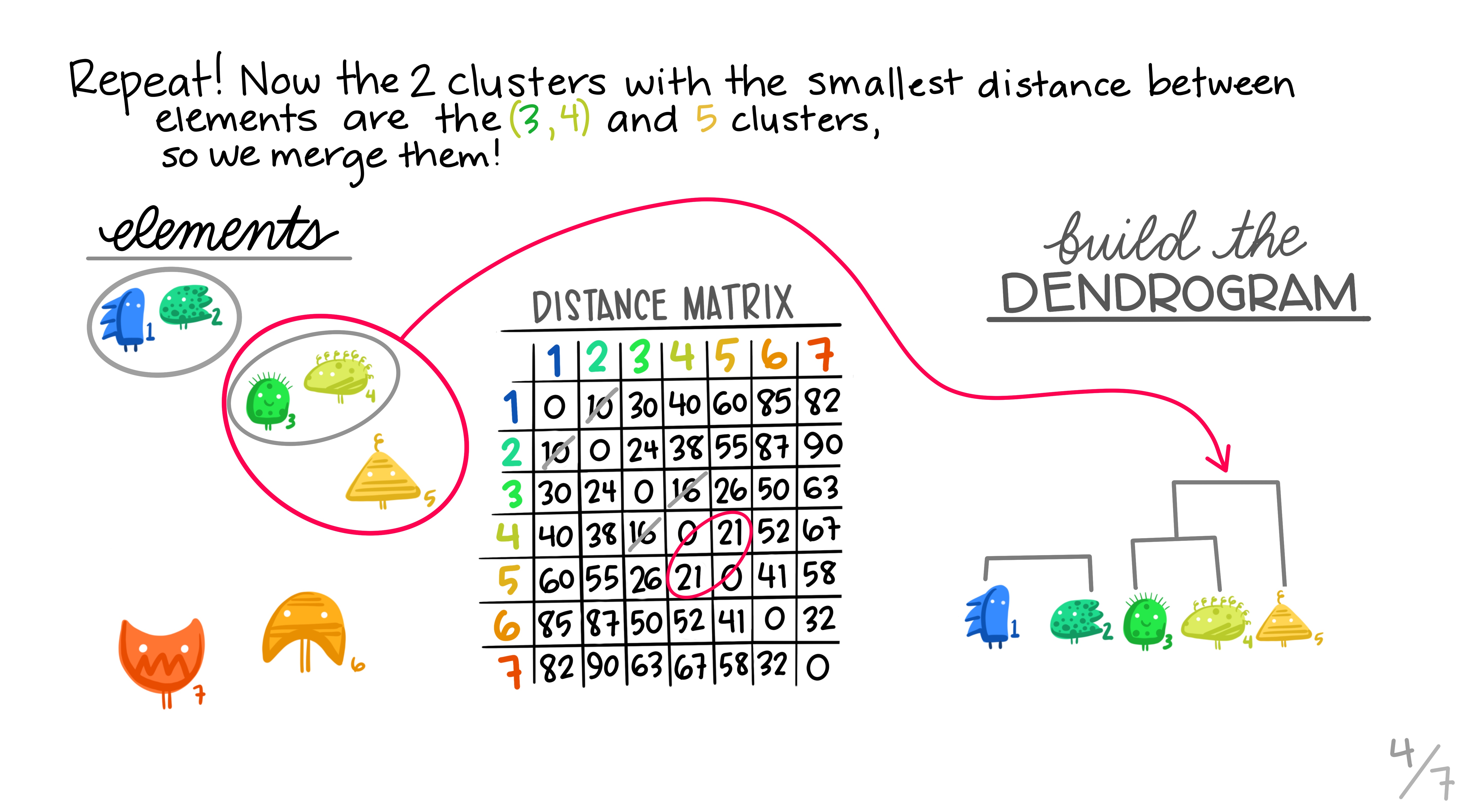
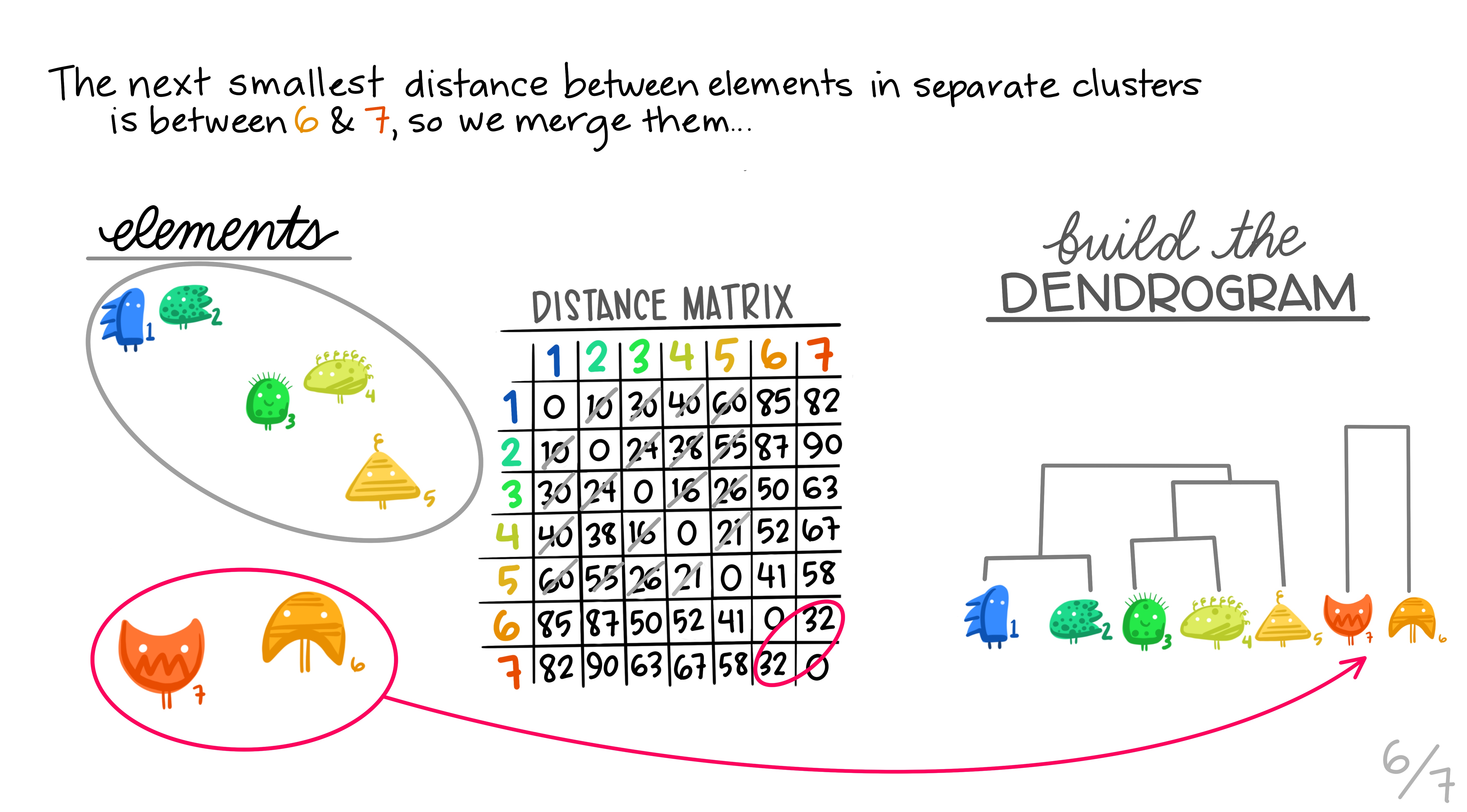
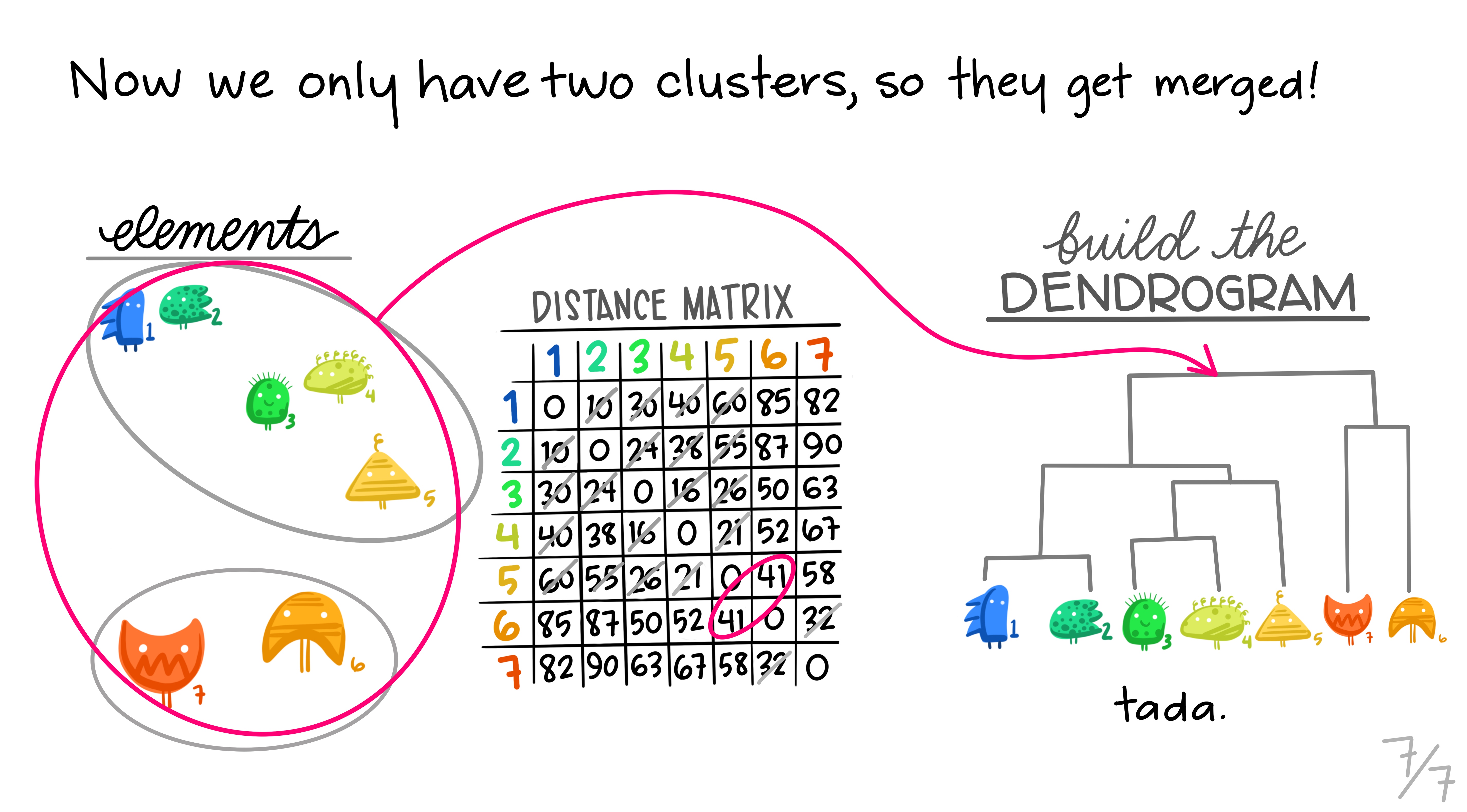
Here are some really nice illustrations explaining how hierarchical cluster analysis is done (Artwork by @allison_horst).
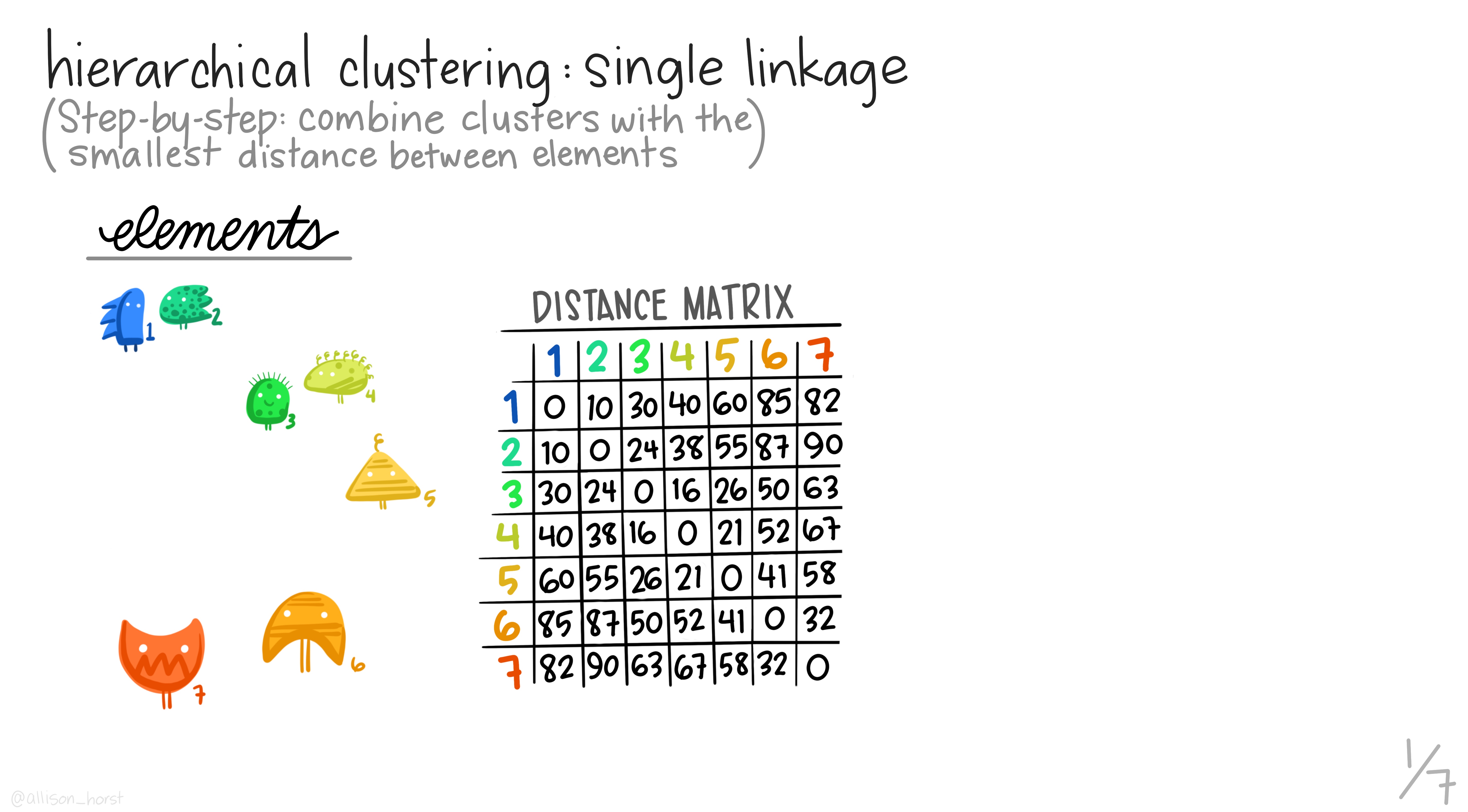
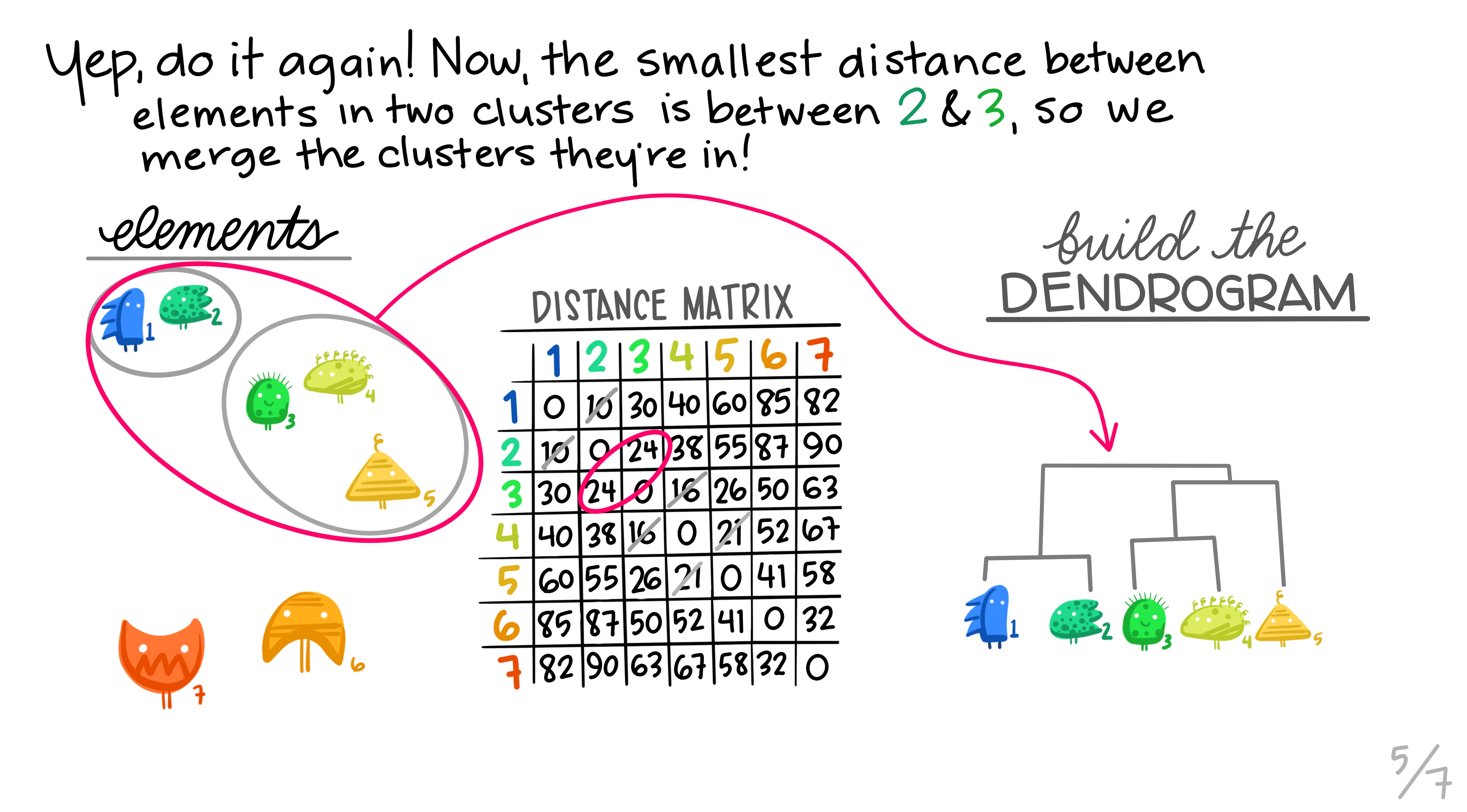
Research context
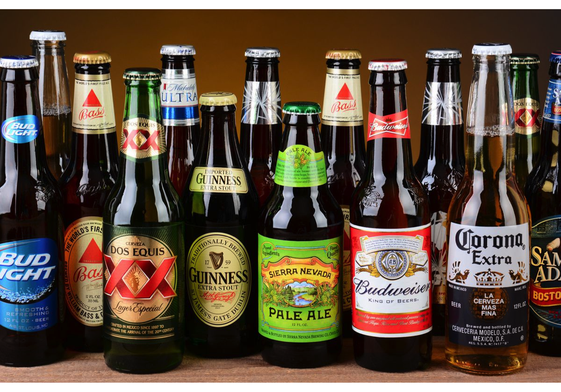
In this example, a marketing analyst is trying to develop a classification scheme for beer based on several characteristics that may be relevant to consumers. She samples 20 popular beers and gathers data on their per-serving in terms of the following 4 aspects:
- calorie content
- sodium content
- alcohol content
- cost per unit volume
Import data
library(EDMS657Data)

head(beer)
## beer calories sodium
## 1 budweiser 144 15
## 2 schlitz 151 19
## 3 lowenbrau 157 15
## 4 knonenbourg 170 7
## 5 heineken 152 11
## 6 old milwaukee 145 23
## alcohol cost
## 1 4.7 0.43
## 2 4.9 0.43
## 3 4.9 0.48
## 4 5.2 0.73
## 5 5.0 0.77
## 6 4.6 0.28describe(beer[,2:5])## vars n mean sd median trimmed mad min max range skew
## calories 1 20 132.40 30.26 144.00 135.19 12.60 68.00 175.00 107.00 -0.77
## sodium 2 20 14.95 6.58 15.00 14.75 6.67 6.00 27.00 21.00 0.17
## alcohol 3 20 4.44 0.76 4.65 4.56 0.52 2.30 5.50 3.20 -1.32
## cost 4 20 0.50 0.14 0.44 0.48 0.04 0.28 0.79 0.51 1.04
## kurtosis se
## calories -0.58 6.77
## sodium -1.30 1.47
## alcohol 1.33 0.17
## cost -0.26 0.03Standardize the data
We need to standardize the 4 variables before we calculate the distance measures.
beer.std <- beer[, 2:5]
beer.std <- apply(beer.std, 2, scale)
Calculate the distances between cases
You can obtain a dissimilarity matrix using the dist()
function. There are different distance measures you could use. In our
example, I am using the Euclidean distance.
(beer.dist <- dist(beer.std, method = "euclidean"))## 1 2 3 4 5 6 7
## 2 0.7015818
## 3 0.6122575 0.7278023
## 4 2.6465145 2.8687653 2.2005449
## 5 2.4877563 2.6626568 2.1174297 0.9327464
## 6 1.6077215 1.2858363 1.9303753 4.1249764 3.9081202
## 7 2.0179228 1.3687686 1.7768847 3.4821062 3.3966309 1.7624153
## 8 1.8321492 1.2474420 1.9073600 3.8470743 3.4646469 1.1630209 1.4402103
## 9 1.7510653 2.3339366 2.2352241 3.3870512 3.0876935 2.7308849 3.6568121
## 10 1.9794263 2.6211123 2.4120328 3.3969229 3.1727380 2.9925141 3.9748312
## 11 0.4974209 0.5621393 0.8699355 2.9102867 2.6144341 1.3576617 1.9104435
## 12 1.6105790 2.0357302 2.1052752 3.4859630 3.0254611 2.3448036 3.3556511
## 13 1.0621014 1.6861707 1.3290052 2.4493901 2.2252804 2.4602902 3.0101426
## 14 2.3829050 2.3108215 2.0702362 2.0586803 1.2816892 3.4004046 2.9393368
## 15 2.8852159 3.1929082 2.5704997 0.8650286 0.7787026 4.4218595 4.0014699
## 16 4.0506915 4.4413426 4.5657715 5.7739101 5.2976396 4.1954211 5.6686729
## 17 0.7715030 0.8239182 1.1853893 3.1703232 2.8239302 1.2711853 2.0924143
## 18 1.3926213 0.7941748 1.4750146 3.4527663 3.0956034 1.1264236 1.3102914
## 19 3.6316284 4.2061309 4.0878395 4.8171366 4.4561667 4.3666086 5.5635455
## 20 2.0978461 2.7268974 2.5026970 3.2900060 3.0227800 3.2328090 4.0598624
## 8 9 10 11 12 13 14
## 2
## 3
## 4
## 5
## 6
## 7
## 8
## 9 3.1120809
## 10 3.3914470 0.9669069
## 11 1.4125349 1.8639961 2.1232552
## 12 2.5374251 0.8365790 1.2489945 1.4958193
## 13 2.6205526 1.3011956 1.1591935 1.2688466 1.2859397
## 14 2.6594018 3.2027807 3.3130407 2.2593417 2.8043925 2.3297032
## 15 4.1184903 3.1968877 3.2191846 3.1012683 3.3099295 2.4432426 2.0254300
## 16 4.5328376 2.9456906 2.6292003 3.8997822 2.6804952 3.4961538 4.9678284
## 17 1.3501679 1.8392272 2.0555040 0.3386672 1.3533428 1.3360762 2.3747645
## 18 0.5560822 2.7130581 3.0756290 1.0046789 2.2246603 2.2530486 2.4403520
## 19 4.7273573 2.1458231 1.7482875 3.6607468 2.3125059 2.8138021 4.5293389
## 20 3.5696841 0.5539882 0.8828019 2.2658231 1.2357508 1.4107464 3.3008172
## 15 16 17 18 19
## 2
## 3
## 4
## 5
## 6
## 7
## 8
## 9
## 10
## 11
## 12
## 13
## 14
## 15
## 16 5.4588664
## 17 3.3137891 3.6305062
## 18 3.7143223 4.4733114 1.0393151
## 19 4.4028558 1.6795526 3.5095654 4.4850403
## 20 3.0067058 3.0069608 2.2655457 3.1640859 1.9074091Alternatively, you could compute the (weighted) Mahalanobis distance using the following function:
library(distances)
beer.mdist <- distances(beer[, 2:5], normalize = "mahalanobize")
Hierarchical cluster analysis
Once you have the dissimilarity measures, you can use the
hclust() function to conduct hierarchical agglomerative
cluster analysis. This function will start off treating each object as
its own cluster. It then examines the distances between all the pairs of
observations and combine the two closest ones to form a new cluster. It
proceeds iteratively joining the two nearest clusters at each step. For
each step, the between-cluster distances are computed based on the
linkage method as the user specified.
Note that you have to manually square the Euclidean distance in order to use the squared Euclidean distance as the distance measures.
(beer.clust <- hclust((beer.dist)^2, method = "ave")) # named "between-groups linkage" in SPSS##
## Call:
## hclust(d = (beer.dist)^2, method = "ave")
##
## Cluster method : average
## Distance : euclidean
## Number of objects: 20You may want to check the clustering/agglomeration schedule to see which cases/clusters were joined at each step. Row i of merge describes the merging of clusters at step i of the clustering. If an element j in the row is negative, then observation -j was merged at this stage. If j is positive then the merge was with the cluster formed at the (earlier) stage j of the algorithm. Thus negative entries in merge indicate agglomerations of singletons, and positive entries indicate agglomerations of non-singletons.
beer.clust$merge## [,1] [,2]
## [1,] -11 -17
## [2,] -9 -20
## [3,] -8 -18
## [4,] -1 -3
## [5,] -2 1
## [6,] -5 -15
## [7,] 4 5
## [8,] -4 6
## [9,] -10 2
## [10,] -12 9
## [11,] -6 3
## [12,] -13 10
## [13,] 7 11
## [14,] -16 -19
## [15,] -7 13
## [16,] -14 8
## [17,] 12 15
## [18,] 16 17
## [19,] 14 18You can also check the clustering heights. It is the distance measure
(using the method as you specified in the hclust()
function) between the two clusters that are joined at each step. When
you see a big jump in the heights, it is a sign suggesting you may not
want to keep those two clusters separate instead of combining them.
# n-1 heights values
beer.clust$height
## [1] 0.1146955 0.3069030 0.3092274 0.3748592 0.4974209 0.6063777
## [7] 0.6710822 0.8091452 0.8571240 1.2623106 1.3107239 1.6701715
## [13] 2.0418729 2.8208970 3.0035036 3.3277528 6.3761856 9.5277574
## [19] 16.9139432# manually compute proportional increase
(prop.height <- beer.clust$height[2:19]/beer.clust$height[1:18])## [1] 2.675806 1.007574 1.212245 1.326954 1.219044 1.106706 1.205732 1.059296
## [9] 1.472728 1.038353 1.274236 1.222553 1.381524 1.064734 1.107957 1.916063
## [17] 1.494272 1.775228schedule <- cbind(beer.clust$merge, beer.clust$height, c(NA,prop.height))
colnames(schedule) <- c("cluster 1", "cluster 2", "height", "proportional increase")
schedule## cluster 1 cluster 2 height proportional increase
## [1,] -11 -17 0.1146955 NA
## [2,] -9 -20 0.3069030 2.675806
## [3,] -8 -18 0.3092274 1.007574
## [4,] -1 -3 0.3748592 1.212245
## [5,] -2 1 0.4974209 1.326954
## [6,] -5 -15 0.6063777 1.219044
## [7,] 4 5 0.6710822 1.106706
## [8,] -4 6 0.8091452 1.205732
## [9,] -10 2 0.8571240 1.059296
## [10,] -12 9 1.2623106 1.472728
## [11,] -6 3 1.3107239 1.038353
## [12,] -13 10 1.6701715 1.274236
## [13,] 7 11 2.0418729 1.222553
## [14,] -16 -19 2.8208970 1.381524
## [15,] -7 13 3.0035036 1.064734
## [16,] -14 8 3.3277528 1.107957
## [17,] 12 15 6.3761856 1.916063
## [18,] 16 17 9.5277574 1.494272
## [19,] 14 18 16.9139432 1.775228You can also visualize the clustering schedule. This is a dendogram (a tree diagram) that you should read from bottom up. The horizontal distances does not mean anything in such diagram. They are programmed to be equally spaced. The y-axis shows you the height values when two clusters are combined. You would not want to join the clusters when you see a huge jump in the height. This dendogram below shows that there are 4 distinct groups.
plot(beer.clust, main = 'Cluster Dendrogram')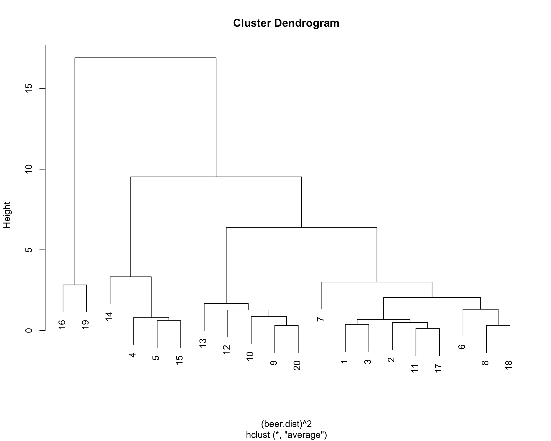
Check the cluster membership
We first cut the tree to keep 4 distince clusters. Then we check the cluster membership of each case and examine the descriptive statistics for each cluster.
(beer.4 <- cutree(beer.clust,4))## [1] 1 1 1 2 2 1 1 1 3 3 1 3 3 2 2 4 1 1 4 3table(beer.4)## beer.4
## 1 2 3 4
## 9 4 5 2# group membership
sapply(unique(beer.4), function(g)beer$beer[beer.4 == g])## [[1]]
## [1] budweiser
## [2] schlitz
## [3] lowenbrau
## [4] old milwaukee
## [5] augsberger
## [6] strohs bohemian
## [7] coors
## [8] hamms
## [9] heilemans old style
## 20 Levels: augsberger ...
##
## [[2]]
## [1] knonenbourg
## [2] heineken
## [3] becks
## [4] kirin
## 20 Levels: augsberger ...
##
## [[3]]
## [1] miller lite
## [2] bud light
## [3] coors light
## [4] michelob light
## [5] schlitz light
## 20 Levels: augsberger ...
##
## [[4]]
## [1] pabst extra light
## [2] olympia gold light
## 20 Levels: augsberger ...# descriptive statistics for each cluster
aggregate(beer[,2:5], by=list(beer.4), mean)## Group.1 calories sodium alcohol cost
## 1 1 149.00 20.44444 4.800 0.4155556
## 2 2 155.25 10.75000 4.975 0.7625000
## 3 3 109.20 10.20000 4.100 0.4600000
## 4 4 70.00 10.50000 2.600 0.4200000aggregate(beer[,2:5], by=list(beer.4), sd)## Group.1 calories sodium alcohol cost
## 1 1 11.510864 4.245913 0.3122499 0.05502525
## 2 2 9.912114 5.909033 0.2061553 0.02500000
## 3 3 15.690762 3.114482 0.2345208 0.02738613
## 4 4 2.828427 6.363961 0.4242641 0.05656854Example 2: K-means Cluster Analysis
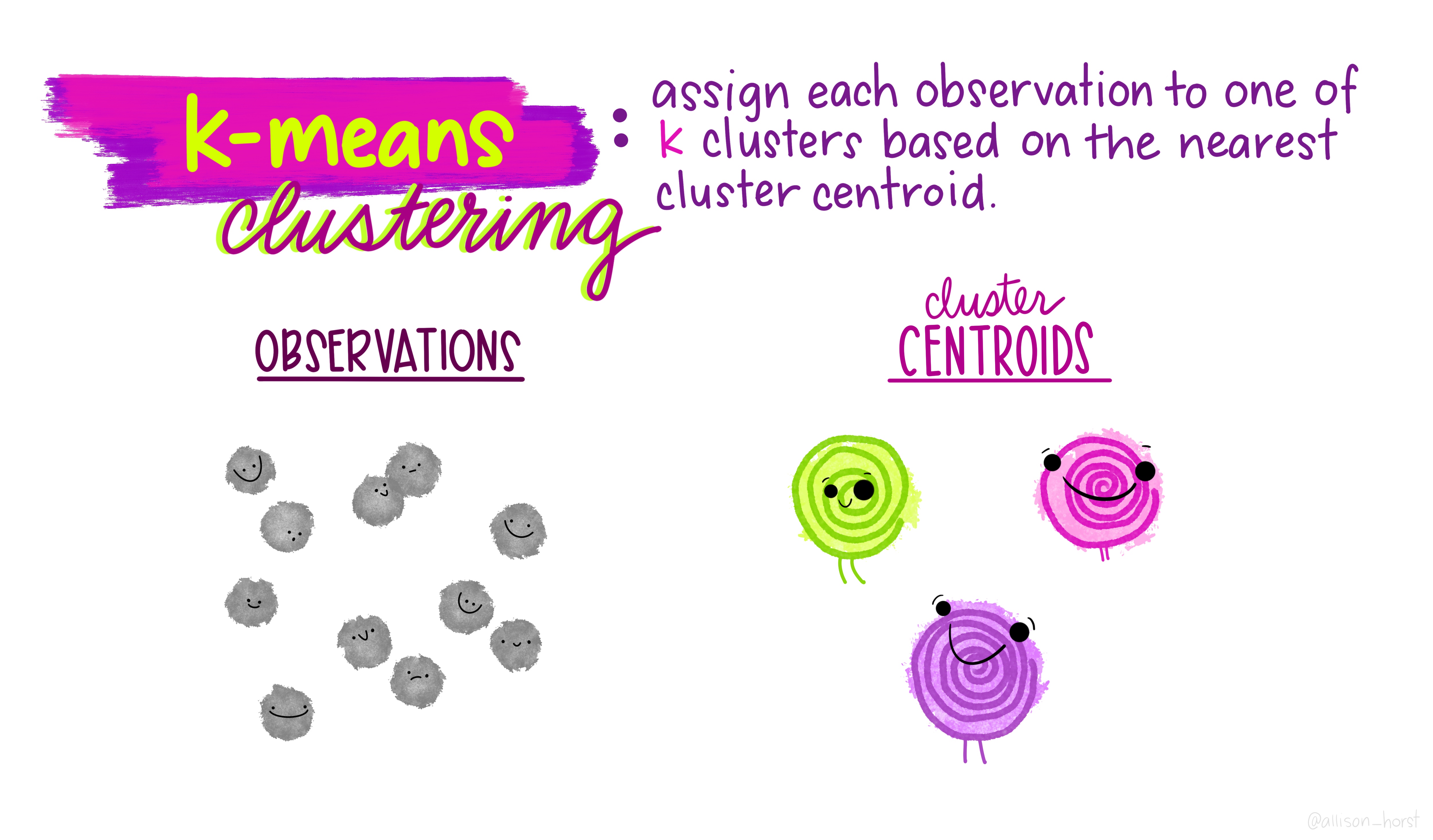
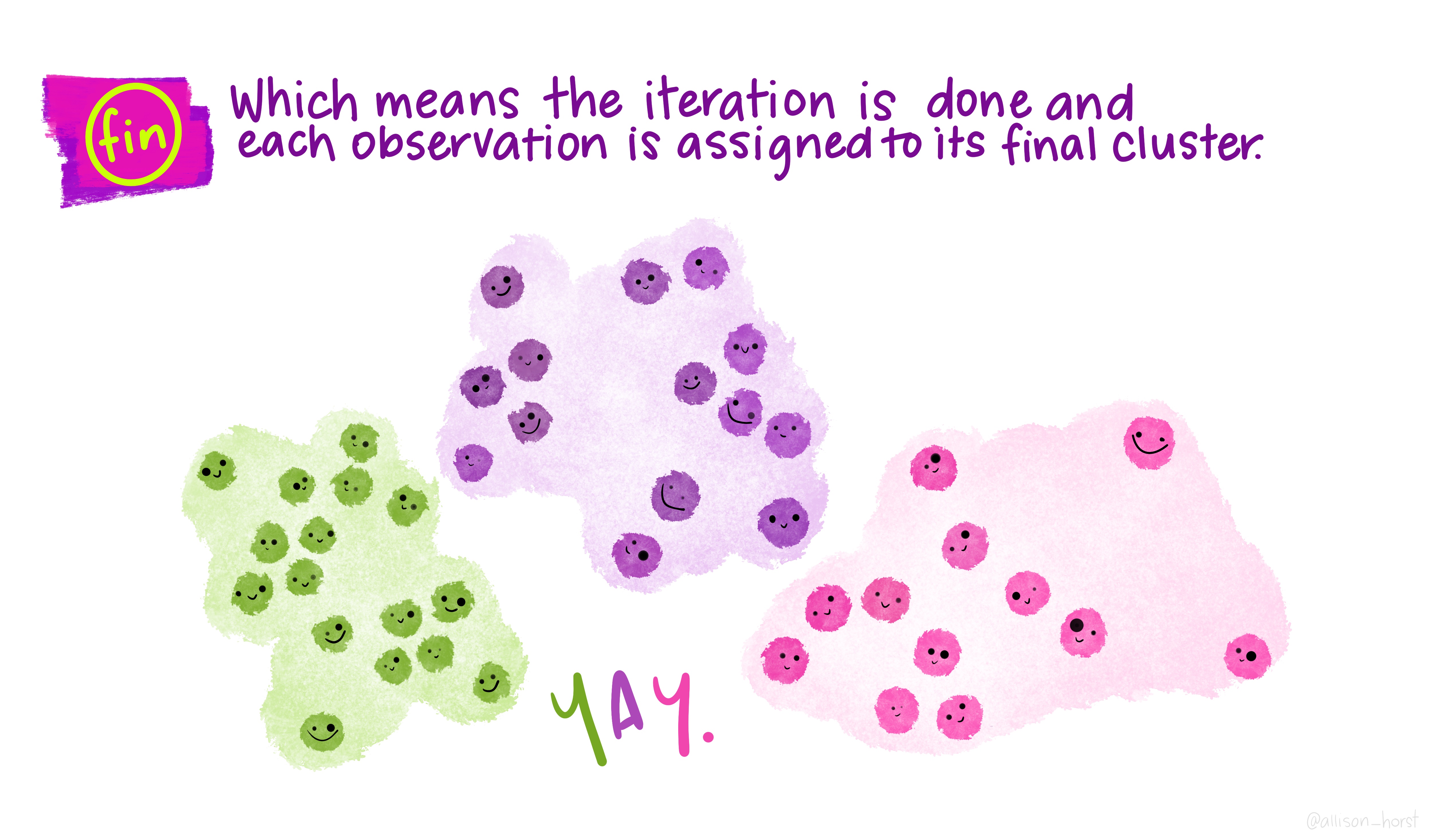
In this example we will demo how to conduct k-means cluster analysis using the Achievement Goal data that were collected from n=2111 college students (see Finney, Pieper, & Barron, 2004).
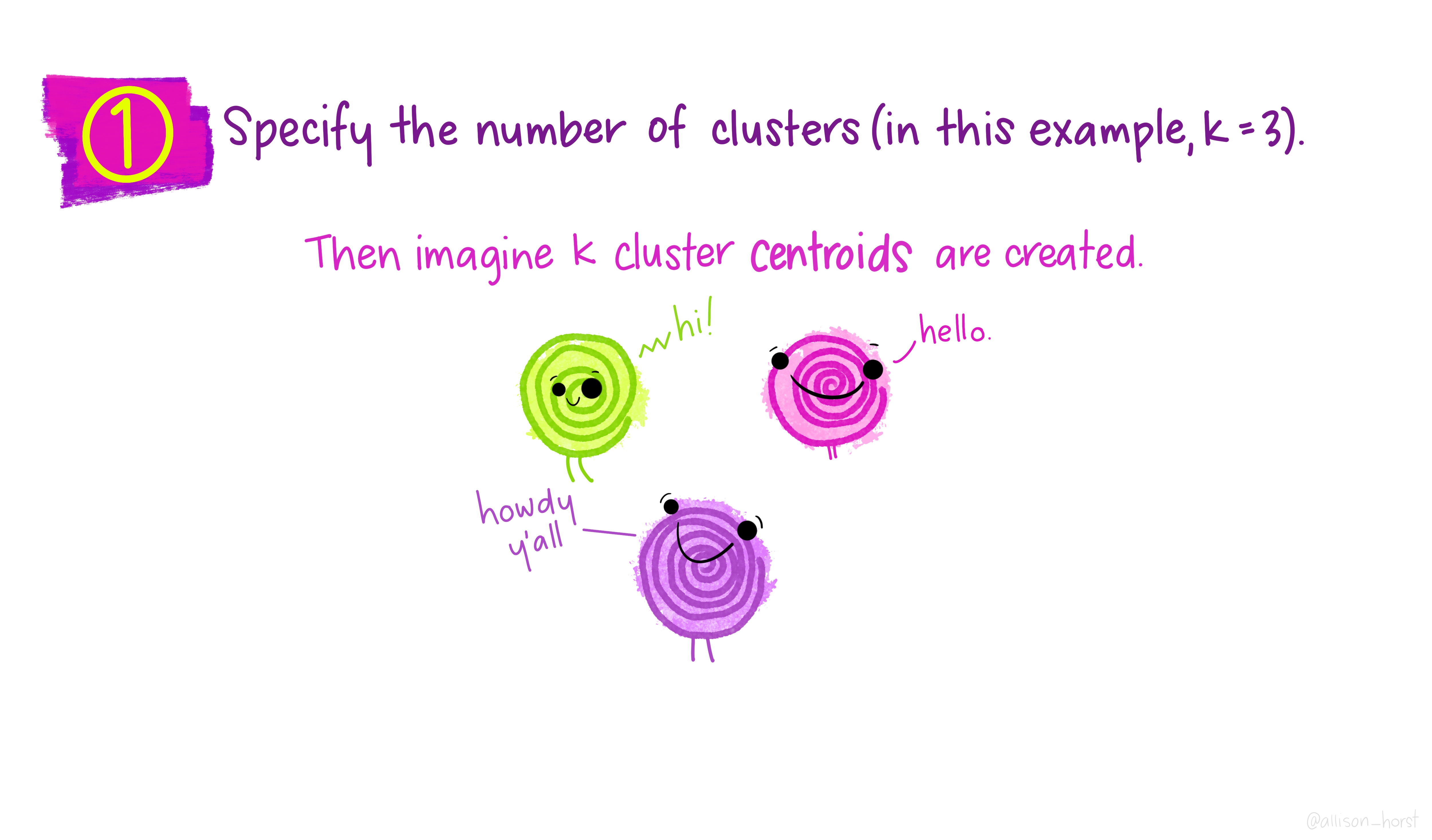
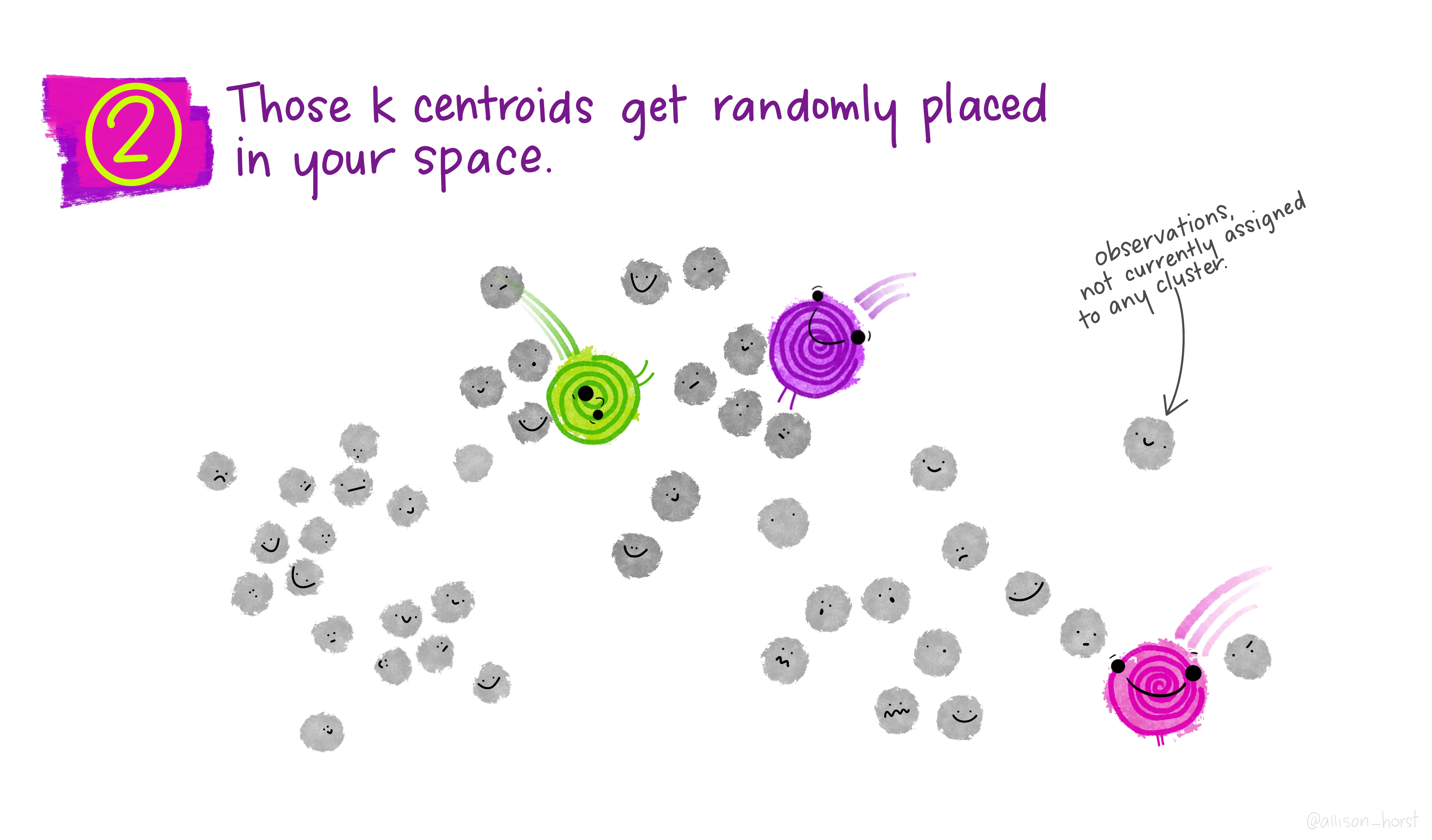
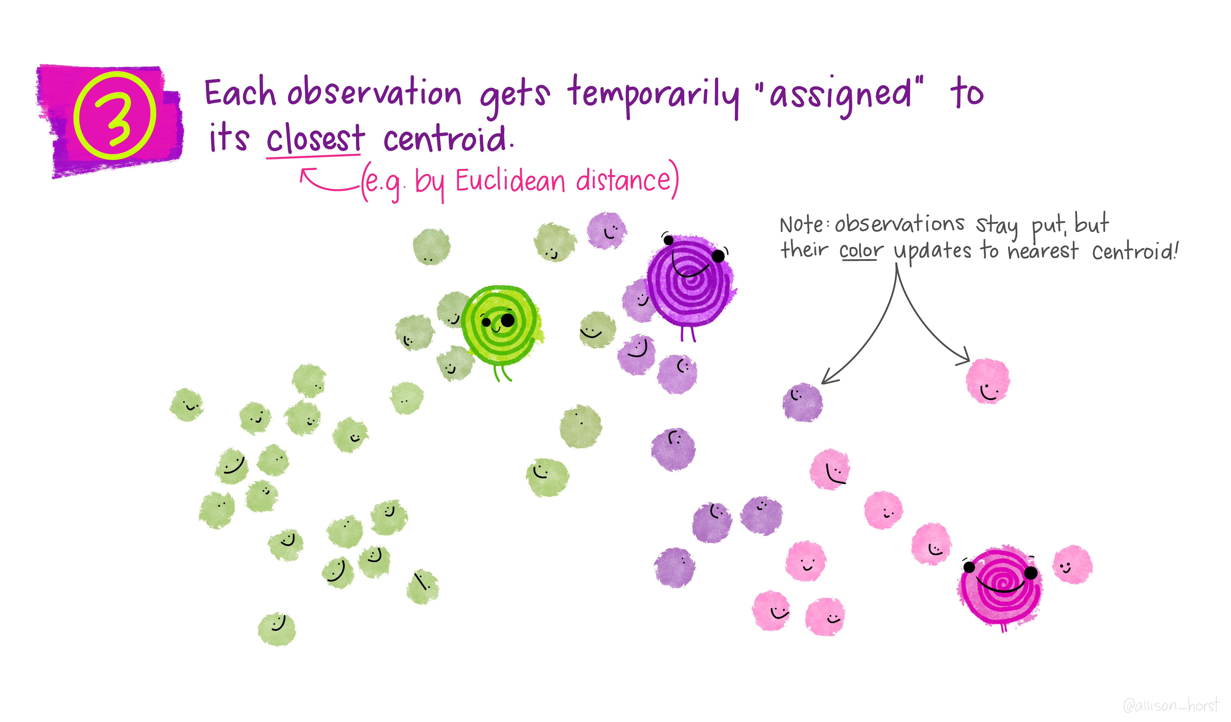
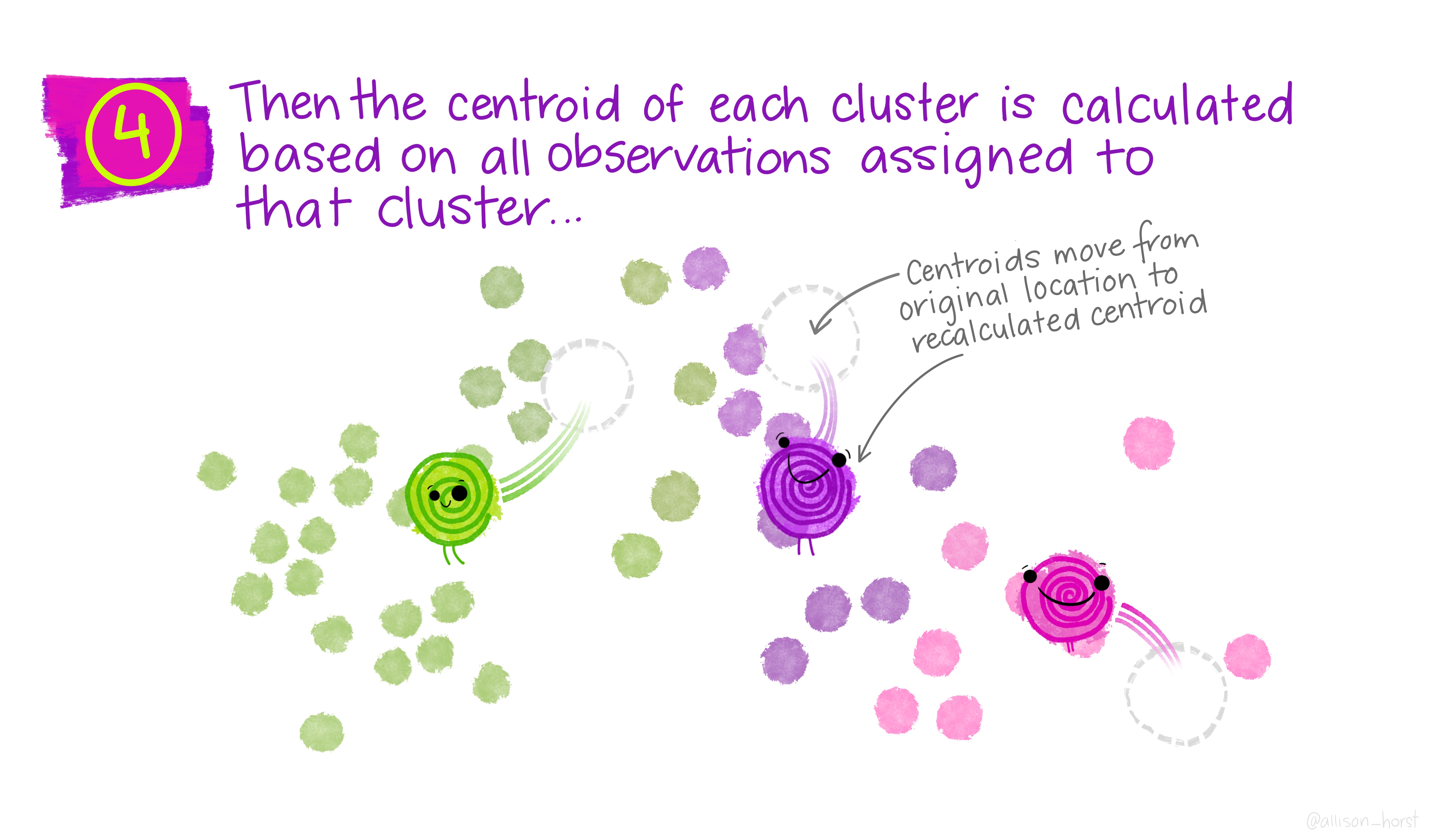
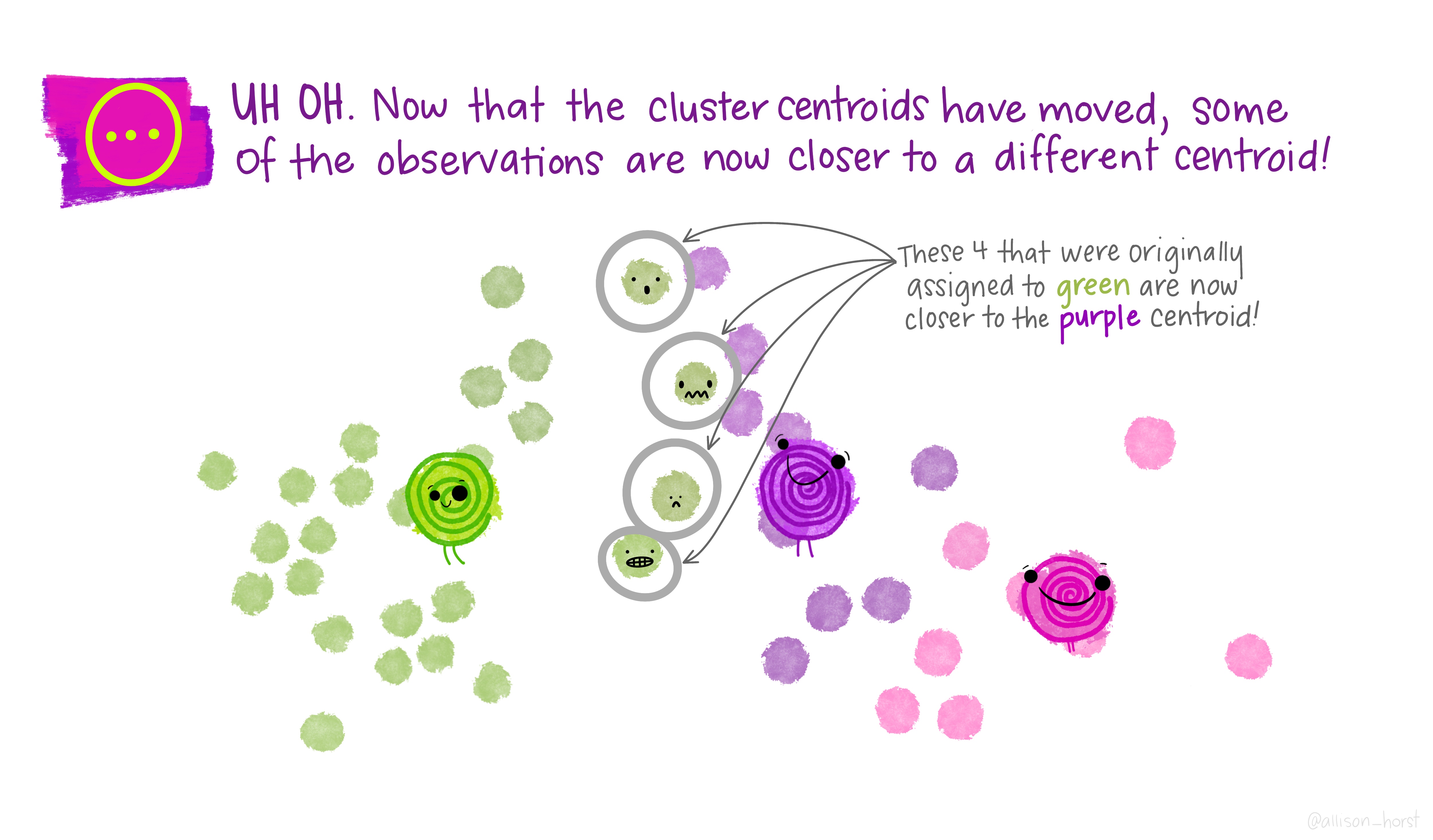
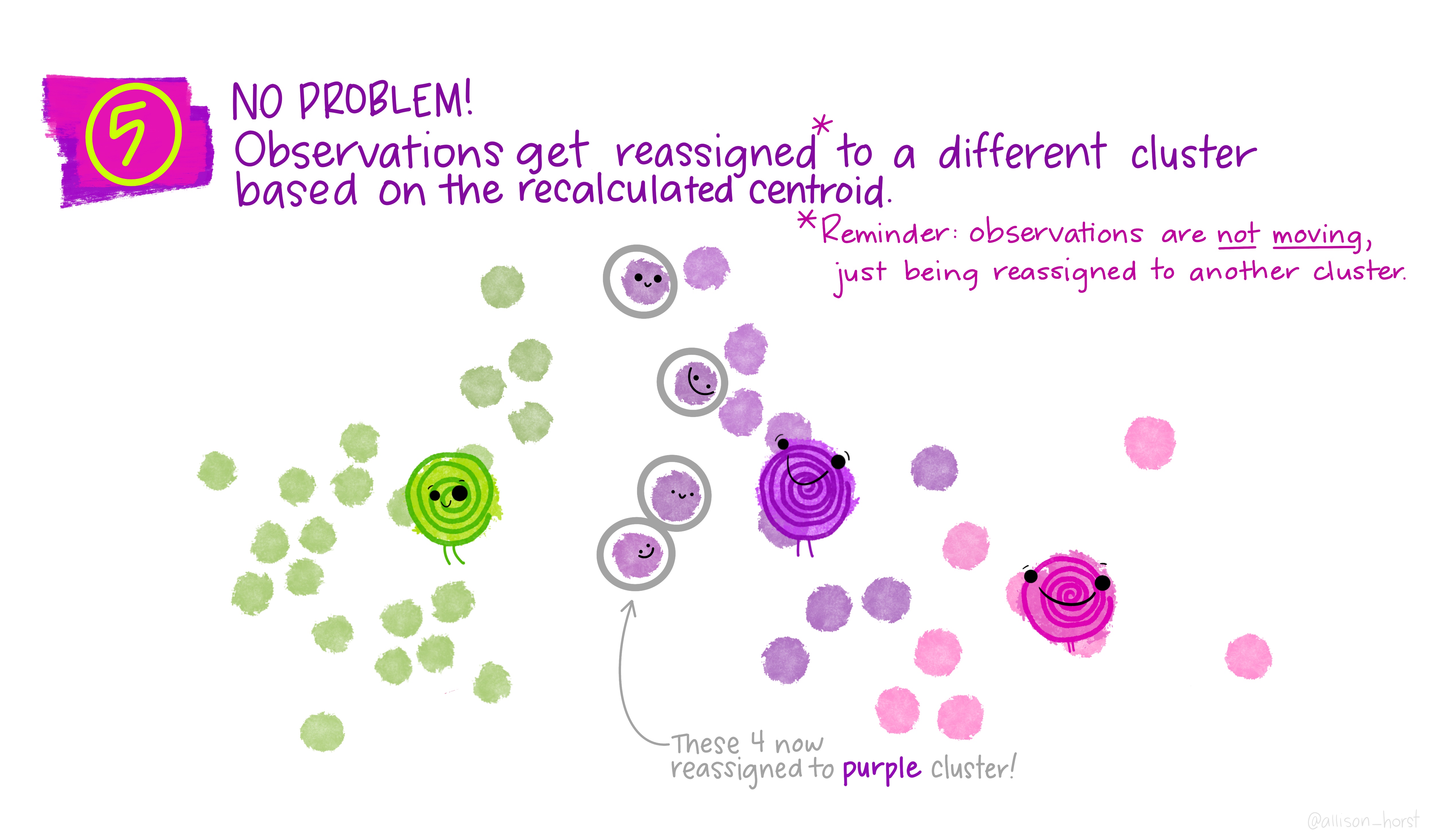
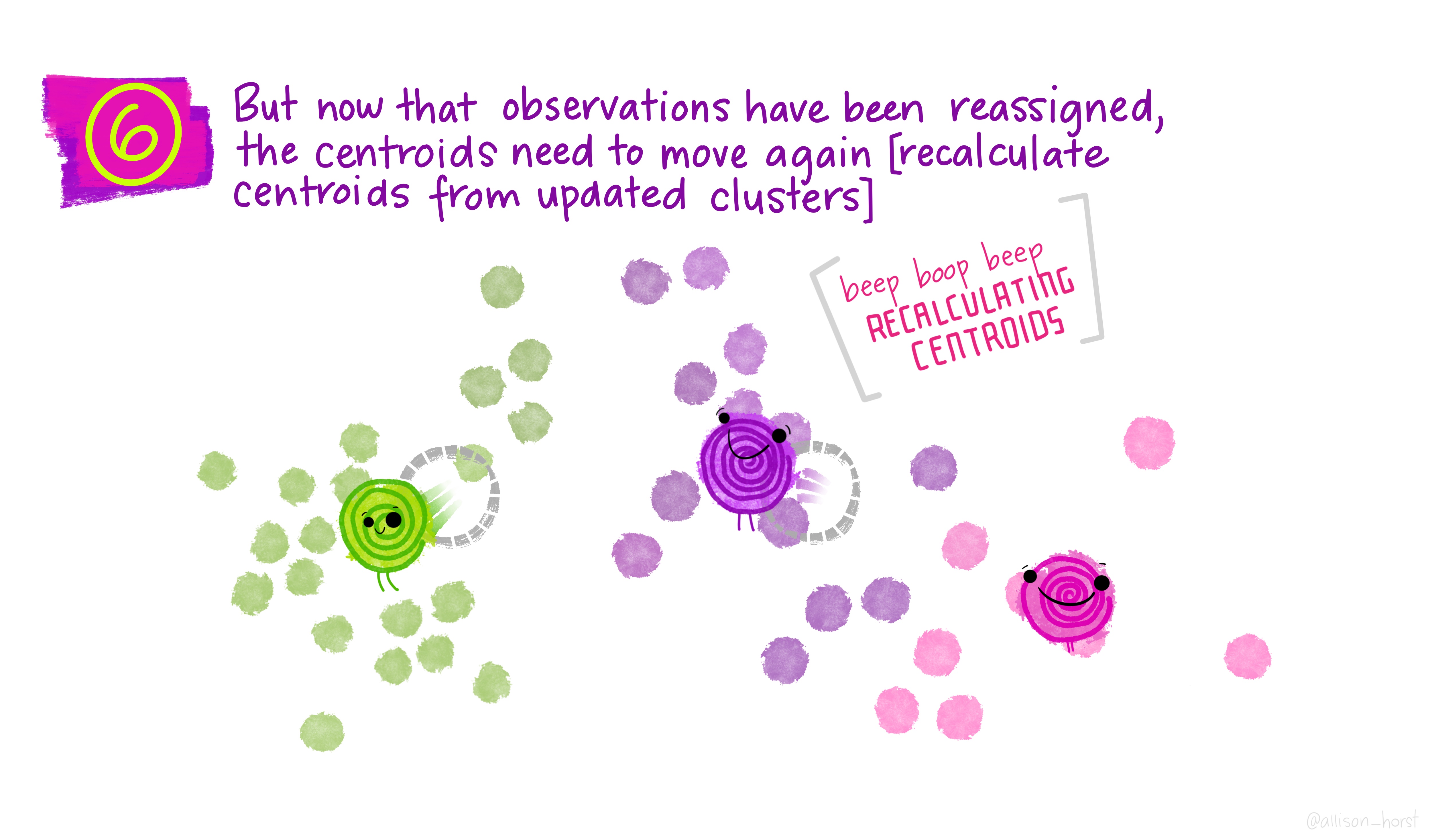
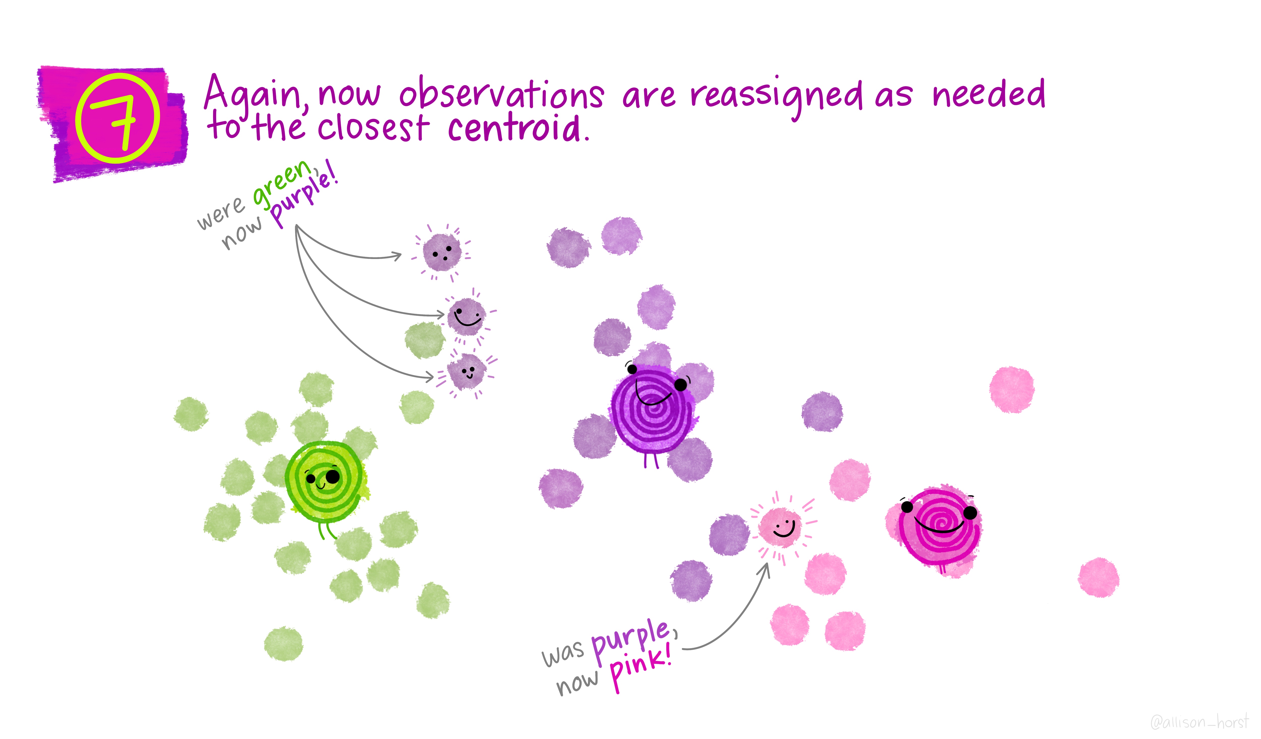
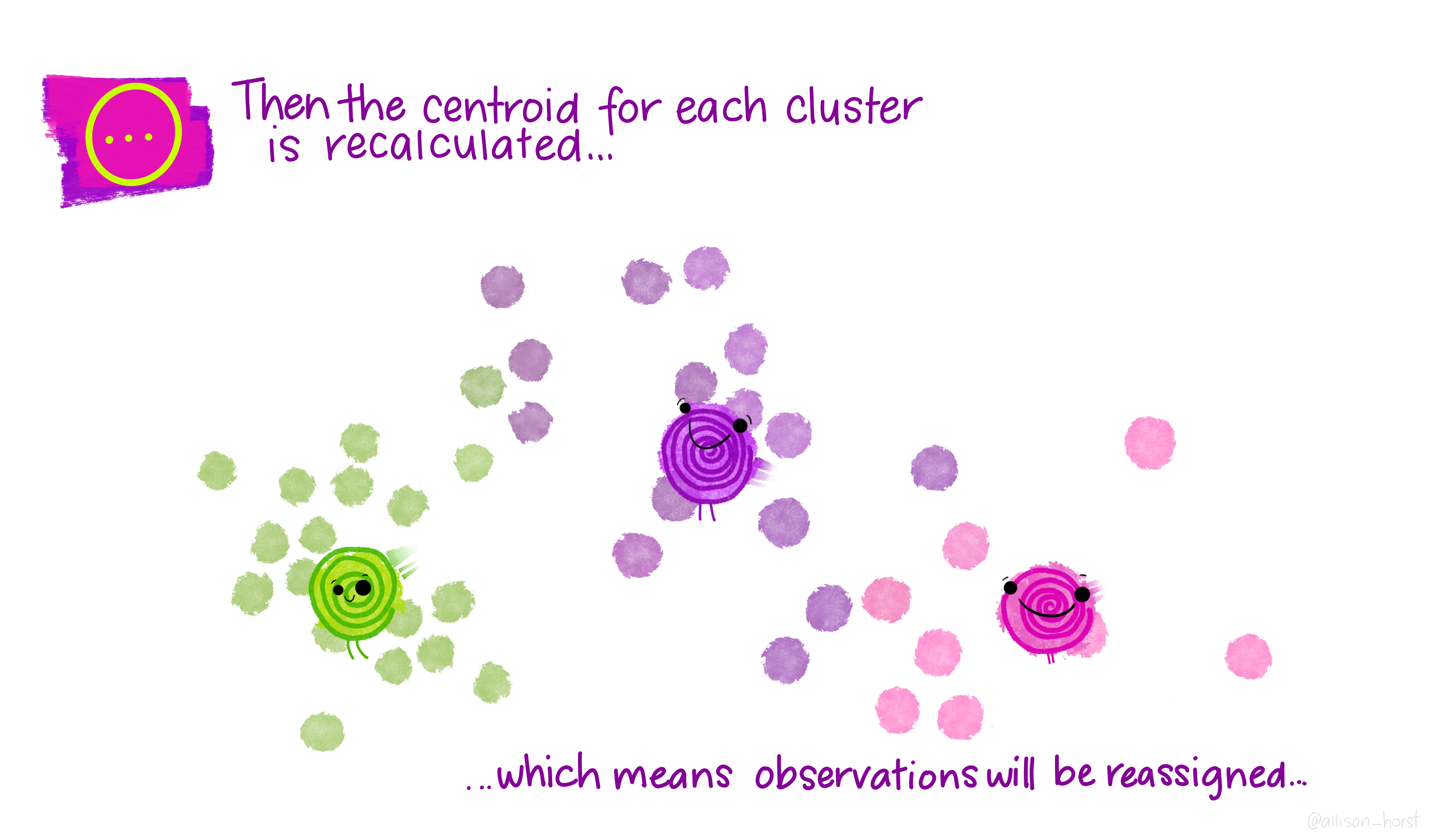
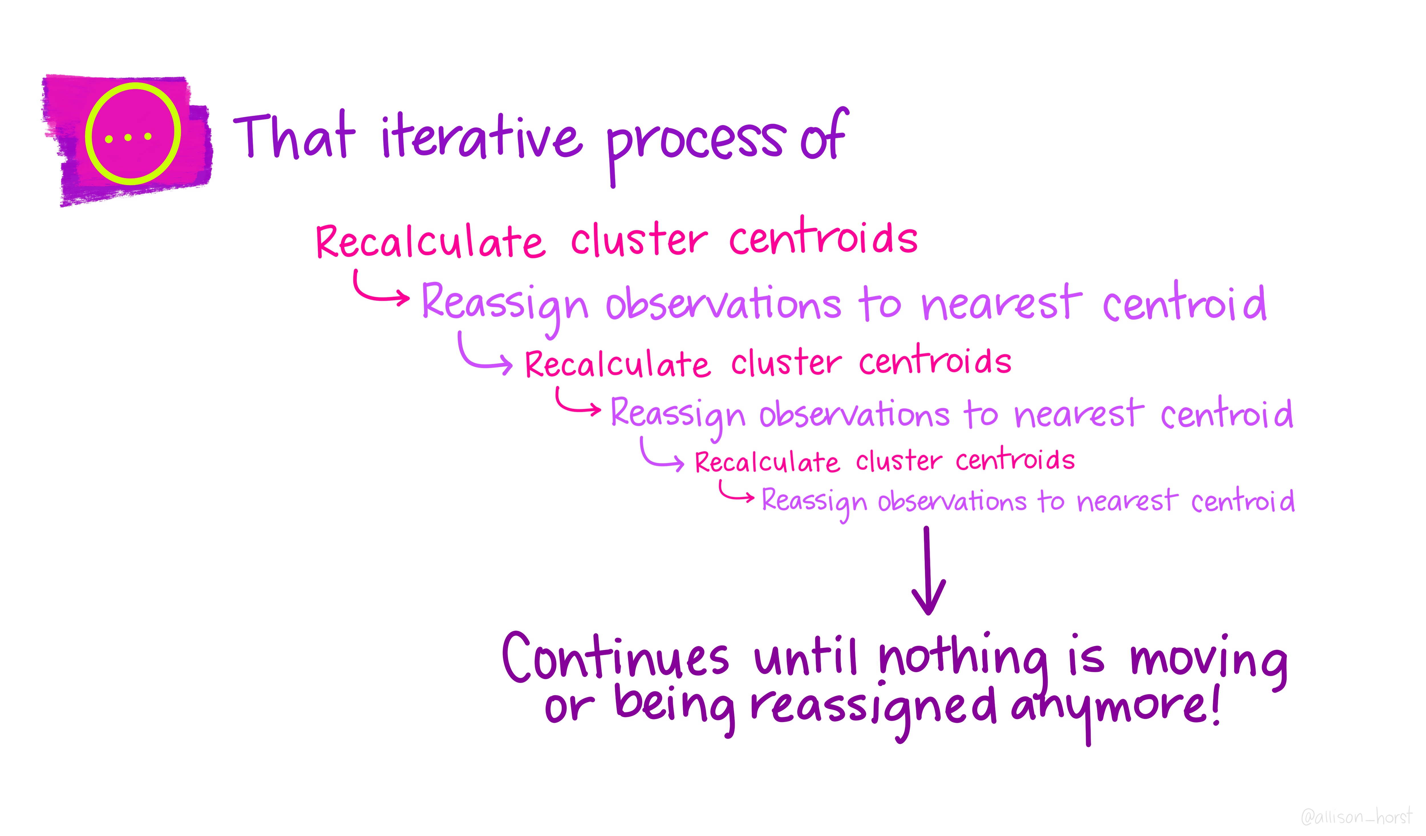
Before we begin, here are some really nice illustrations explaining how k-means cluster analysis is done (Artwork by @allison_horst).
Import Data
Let’s first take a look at the data:
library(EDMS657Data)
head(AGOscores)
## MAP PAP PAV MAV ID
## 1 18 21 8 7 1
## 2 13 14 13 17 2
## 3 14 15 11 17 3
## 4 21 21 8 19 4
## 5 19 17 8 16 5
## 6 20 21 3 4 6str(AGOscores)## 'data.frame': 1868 obs. of 5 variables:
## $ MAP: int 18 13 14 21 19 20 16 14 13 8 ...
## $ PAP: int 21 14 15 21 17 21 15 17 11 11 ...
## $ PAV: int 8 13 11 8 8 3 14 12 8 8 ...
## $ MAV: int 7 17 17 19 16 4 16 14 9 9 ...
## $ ID : int 1 2 3 4 5 6 7 8 9 10 ...Standardize the data
We need to standardize the variables before we implement cluster analysis.
AGO.std <- AGOscores[, 1:4]
AGO.std <- apply(AGO.std, 2, scale)
How many clusters?
Next we could use the fviz_nbclust function from the
factoextra package to help us determine the number of
clusters we would like to specify. You could use different criterion for
selecting the number of clusters. Here I am using the total within sum
of square (WSS) as my criterion.
library(factoextra)

fviz_nbclust(AGO.std, FUNcluster = kmeans, method = "wss") +
geom_vline(xintercept = 5, linetype = 2)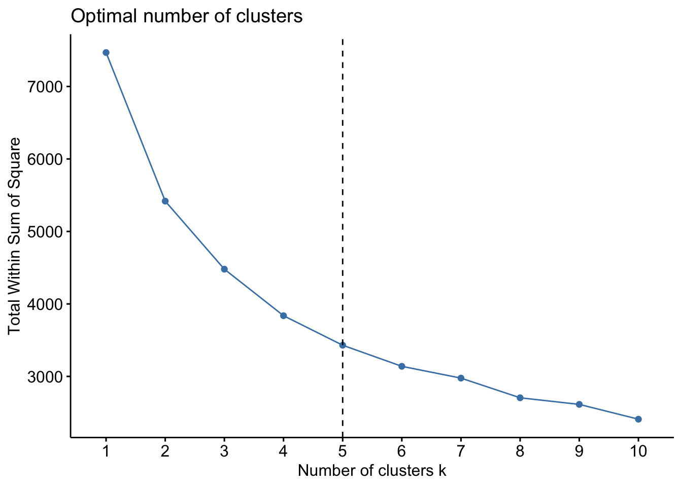
K-means clustering
We could then conduct k-means clustering with 5 clusters. We specify
nstart = 25. This means that we want R to try 25 different
random initial assignment and then select the best results that yield
the lowest WSS.
The output of kmeans() is a list containing the
following components:
cluster: A vector of integers (from 1:k) indicating the cluster to which each point is allocated.centers: A matrix of cluster centers.totss: The total sum of squares.withinss: Vector of within-cluster sum of squares, one component per cluster.tot.withinss: Total within-cluster sum of squares, i.e. sum(withinss).betweenss: The between-cluster sum of squares.size: The number of points in each cluster.
km_5 <- stats::kmeans(AGO.std, centers = 5, nstart = 25)

km_5$size
## [1] 357 414 311 264 522km_5$centers## MAP PAP PAV MAV
## 1 0.35451787 0.6432040 -0.5069146 0.82212556
## 2 -1.31450993 -0.4160773 -0.3644845 -0.02860851
## 3 0.53676877 0.5230574 -0.6749074 -1.07426218
## 4 -0.01423878 -1.6156389 -0.1518589 -0.98703186
## 5 0.48748694 0.3955747 1.1146591 0.59964952Visualize the results
We could visualize the k-means clustering results using the
fviz_cluster function.
factoextra::fviz_cluster(km_5, AGO.std, geom = "point")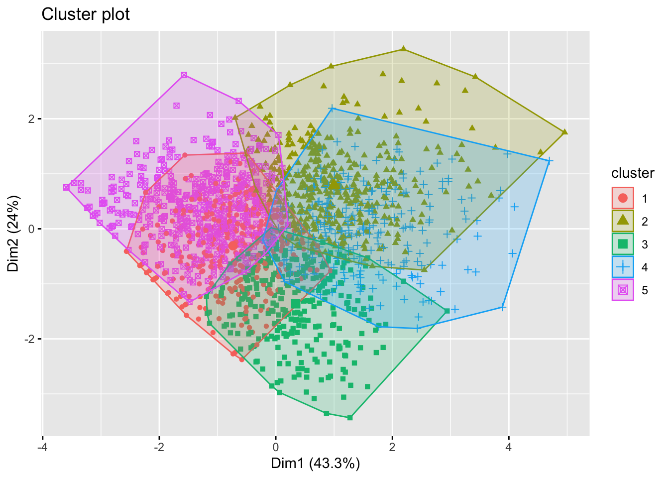
The R script for this tutorial can be found here.
© Copyright 2022 Yi Feng and Gregory R. Hancock.