EDMS 657-R Tutorial: EFA with Polytomous Data
Yi Feng & Gregory R. Hancock
University of Maryland, College ParkIn this document we will show how to conduct EFA with polytomous data using R. This document serves as a supplementary material for EDMS 657-Exploratory Latent and Composite Variable Methods, taught by Dr. Gregory R. Hancock at University of Maryland.
First let us make sure we have installed and loaded the R packages that are used for this demo.
install.packages("psych")
install.packages("devtools")
devtools::install_github("YiFengEDMS/EDMS657Data")
library(psych)
library(EDMS657Data)Research Context
Finney et al. (2004) pilot-tested four scale items that are expected to measure a single factor: Working Avoidance Orientation.
The four items are are listed below:
- V1: “I want to do as little work as possible this semester.”
- V2: “I really don’t want to work hard in my classes in this semester.”
- V3: “I want to get through my courses by doing the least amount of work possible.”
- V4: “I look forward to working really hard this semester in my coursework.” (reverse coded)
For this example, the responses were coded on a 3-point scale (1 = not true, 3 = very true), \(n=300\). We are interested in investigating the underlying latent factor(s) measured by the above four items.
Check the Data
wav2 <- wav
wav2[, 1:4] <- lapply(wav2[, 1:4], as.factor)

head(wav2)
## V1 V2 V3 V4
## 1 1 1 1 1
## 2 1 2 2 2
## 3 1 1 1 1
## 4 1 1 1 1
## 5 3 2 2 2
## 6 1 2 2 2summary(wav2)## V1 V2 V3 V4
## 1:184 1:159 1:164 1:112
## 2:101 2:123 2:117 2:164
## 3: 15 3: 18 3: 19 3: 24str(wav2)## 'data.frame': 300 obs. of 4 variables:
## $ V1: Factor w/ 3 levels "1","2","3": 1 1 1 1 3 1 2 1 1 2 ...
## $ V2: Factor w/ 3 levels "1","2","3": 1 2 1 1 2 2 2 1 1 2 ...
## $ V3: Factor w/ 3 levels "1","2","3": 1 2 1 1 2 2 2 2 1 1 ...
## $ V4: Factor w/ 3 levels "1","2","3": 1 2 1 1 2 2 2 2 1 2 ...The responese are on an ordinal scale and thus it is imprudent to conduct EFA using the bivariate Pearson correlations. Generally speaking, it is more straightforward to conduct EFA with polytomous data within Mplus than within R. While it is a one-step procedure using Mplus, you need to manually go through two steps in R.
Estimate the Polychoric Correlations
We first need to estimate the polychoric correlations using the
mixedCor function to find the polychoric correlations.
(wav.cor <- mixedCor(wav, c = NULL, p = 1:4))## Call: mixedCor(data = wav, c = NULL, p = 1:4)
## V1 V2 V3 V4
## V1 1.00
## V2 0.74 1.00
## V3 0.70 0.75 1.00
## V4 0.59 0.49 0.49 1.00str(wav.cor)## List of 6
## $ rho : num [1:4, 1:4] 1 0.743 0.696 0.586 0.743 ...
## ..- attr(*, "dimnames")=List of 2
## .. ..$ : chr [1:4] "V1" "V2" "V3" "V4"
## .. ..$ : chr [1:4] "V1" "V2" "V3" "V4"
## $ rx : NULL
## $ poly :List of 5
## ..$ rho : num [1:4, 1:4] 1 0.743 0.696 0.586 0.743 ...
## .. ..- attr(*, "dimnames")=List of 2
## .. .. ..$ : chr [1:4] "V1" "V2" "V3" "V4"
## .. .. ..$ : chr [1:4] "V1" "V2" "V3" "V4"
## ..$ tau : num [1:4, 1:2] 0.288 0.0753 0.1172 -0.323 1.6449 ...
## .. ..- attr(*, "dimnames")=List of 2
## .. .. ..$ : chr [1:4] "V1" "V2" "V3" "V4"
## .. .. ..$ : chr [1:2] "1" "2"
## ..$ tauy : NULL
## ..$ n.obs: int 300
## ..$ Call : language polychoric(x = data[, p], smooth = smooth, global = global, weight = weight, correct = correct)
## ..- attr(*, "class")= chr [1:2] "psych" "poly"
## $ tetra:List of 2
## ..$ rho: NULL
## ..$ tau: NULL
## $ rpd : NULL
## $ Call : language mixedCor(data = wav, c = NULL, p = 1:4)
## - attr(*, "class")= chr [1:2] "psych" "mixed"The polychoric correlations can be extracted from the results:
(wav.poly <- wav.cor$rho)## V1 V2 V3 V4
## V1 1.0000000 0.7429990 0.6962313 0.5862258
## V2 0.7429990 1.0000000 0.7509002 0.4862118
## V3 0.6962313 0.7509002 1.0000000 0.4883686
## V4 0.5862258 0.4862118 0.4883686 1.0000000EFA with Polychoric Correlations
Next, we use the polychoric correlations found at step 1 as our data
and proceed with EFA using the fa function. But we need to
specify cor='poly' in the case of polytomous data.
scree(wav.poly)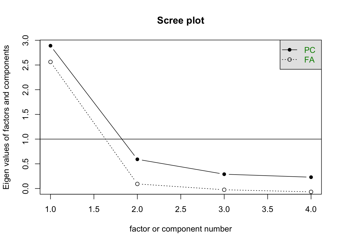
(wav.fa1 <- fa(wav.poly, n.obs = 300, nfactors = 1, fm = 'ml', rotate = 'none', cor = 'poly'))## Factor Analysis using method = ml
## Call: fa(r = wav.poly, nfactors = 1, n.obs = 300, rotate = "none",
## fm = "ml", cor = "poly")
## Standardized loadings (pattern matrix) based upon correlation matrix
## ML1 h2 u2 com
## V1 0.85 0.73 0.27 1
## V2 0.87 0.76 0.24 1
## V3 0.84 0.70 0.30 1
## V4 0.61 0.37 0.63 1
##
## ML1
## SS loadings 2.56
## Proportion Var 0.64
##
## Mean item complexity = 1
## Test of the hypothesis that 1 factor is sufficient.
##
## The degrees of freedom for the null model are 6 and the objective function was 2.18 with Chi Square of 646.24
## The degrees of freedom for the model are 2 and the objective function was 0.05
##
## The root mean square of the residuals (RMSR) is 0.04
## The df corrected root mean square of the residuals is 0.06
##
## The harmonic number of observations is 300 with the empirical chi square 4.59 with prob < 0.1
## The total number of observations was 300 with Likelihood Chi Square = 15.03 with prob < 0.00054
##
## Tucker Lewis Index of factoring reliability = 0.939
## RMSEA index = 0.147 and the 90 % confidence intervals are 0.084 0.221
## BIC = 3.63
## Fit based upon off diagonal values = 1
## Measures of factor score adequacy
## ML1
## Correlation of (regression) scores with factors 0.95
## Multiple R square of scores with factors 0.90
## Minimum correlation of possible factor scores 0.80wav.fa1$loadings##
## Loadings:
## ML1
## V1 0.854
## V2 0.874
## V3 0.836
## V4 0.606
##
## ML1
## SS loadings 2.561
## Proportion Var 0.640You can also try a 2-factor solution with or without rotation.
#2-factor solution
(wav.fa2 <- fa(wav.poly, n.obs = 300, nfactors = 2, fm = 'ml', rotate = 'none', cor = 'poly')) #no rotation
## Factor Analysis using method = ml
## Call: fa(r = wav.poly, nfactors = 2, n.obs = 300, rotate = "none",
## fm = "ml", cor = "poly")
## Standardized loadings (pattern matrix) based upon correlation matrix
## ML1 ML2 h2 u2 com
## V1 0.85 0.24 0.78 0.22 1.2
## V2 0.93 -0.17 0.89 0.11 1.1
## V3 0.82 0.02 0.67 0.33 1.0
## V4 0.59 0.35 0.47 0.53 1.6
##
## ML1 ML2
## SS loadings 2.59 0.21
## Proportion Var 0.65 0.05
## Cumulative Var 0.65 0.70
## Proportion Explained 0.92 0.08
## Cumulative Proportion 0.92 1.00
##
## Mean item complexity = 1.2
## Test of the hypothesis that 2 factors are sufficient.
##
## The degrees of freedom for the null model are 6 and the objective function was 2.18 with Chi Square of 646.24
## The degrees of freedom for the model are -1 and the objective function was 0
##
## The root mean square of the residuals (RMSR) is 0
## The df corrected root mean square of the residuals is NA
##
## The harmonic number of observations is 300 with the empirical chi square 0 with prob < NA
## The total number of observations was 300 with Likelihood Chi Square = 0 with prob < NA
##
## Tucker Lewis Index of factoring reliability = 1.009
## Fit based upon off diagonal values = 1
## Measures of factor score adequacy
## ML1 ML2
## Correlation of (regression) scores with factors 0.96 0.66
## Multiple R square of scores with factors 0.93 0.43
## Minimum correlation of possible factor scores 0.86 -0.14(wav.fa2.pro <- fa(wav.poly, n.obs = 300, nfactors = 2, fm = 'ml', rotate = 'promax', cor = 'poly')) #promax rotation## Factor Analysis using method = ml
## Call: fa(r = wav.poly, nfactors = 2, n.obs = 300, rotate = "promax",
## fm = "ml", cor = "poly")
## Standardized loadings (pattern matrix) based upon correlation matrix
## ML1 ML2 h2 u2 com
## V1 0.33 0.60 0.78 0.22 1.6
## V2 0.98 -0.05 0.89 0.11 1.0
## V3 0.62 0.23 0.67 0.33 1.3
## V4 -0.03 0.71 0.47 0.53 1.0
##
## ML1 ML2
## SS loadings 1.67 1.13
## Proportion Var 0.42 0.28
## Cumulative Var 0.42 0.70
## Proportion Explained 0.60 0.40
## Cumulative Proportion 0.60 1.00
##
## With factor correlations of
## ML1 ML2
## ML1 1.00 0.79
## ML2 0.79 1.00
##
## Mean item complexity = 1.2
## Test of the hypothesis that 2 factors are sufficient.
##
## The degrees of freedom for the null model are 6 and the objective function was 2.18 with Chi Square of 646.24
## The degrees of freedom for the model are -1 and the objective function was 0
##
## The root mean square of the residuals (RMSR) is 0
## The df corrected root mean square of the residuals is NA
##
## The harmonic number of observations is 300 with the empirical chi square 0 with prob < NA
## The total number of observations was 300 with Likelihood Chi Square = 0 with prob < NA
##
## Tucker Lewis Index of factoring reliability = 1.009
## Fit based upon off diagonal values = 1
## Measures of factor score adequacy
## ML1 ML2
## Correlation of (regression) scores with factors 0.96 0.90
## Multiple R square of scores with factors 0.92 0.81
## Minimum correlation of possible factor scores 0.84 0.62wav.fa2.pro$Phi #correlations between the factors## ML1 ML2
## ML1 1.0000000 0.7901203
## ML2 0.7901203 1.0000000Model Fit
Although it is less common to check on model fit in EFA compared to CFA, you can still look at the model fit indicies and have some ideas about how good your solution fits the data. Here is some fit indices for the 1-factor solution.
wav.fa1$chi # Empirical Chi-square## [1] 4.593291wav.fa1$STATISTIC # Likelihood Chi-square statistic## [1] 15.03286wav.fa1$rms # root mean square residual (called SRMR in Mplus), sum of the squared (off diagonal residuals) divided by the degrees of freedom## [1] 0.03571994The psych package outputs a variety of model fit
indicies by default. For example, it calculates two \(\chi^2\) test statistics: the empirical
\(\chi^2\) and the likelihood \(\chi^2\). Where are they from? The
likelihood \(\chi^2\) in
psych package is computed using the following formula:
\[\chi^2 = (n.obs - 1 - \frac{2 \times p + 5}{6} - \frac{2 \times n.factors}{3})\times f,\] where \(p\) is the number of observed variables, and \(f\) is the value of the fitting function.
In brief, the fitting function gauges how far the model-implied correlations are from the observed sample correlations. Assuming multivariate normality, unit variance for the latent factors, and no oblique rotation, the ML fitting function is usually the following (note that their documentation has this formula wrong):
\[f=F_{ML}=\text{tr} ((\textbf{L}\textbf{L}'+\textbf{U})^{-1} \textbf{S}) - \text{ln}(|(\textbf{L}\textbf{L}'+\textbf{U})^{-1} \textbf{S}|) - p,\] where \(\textbf{L}\) is the factor loading matrix, \(\textbf{U}\) is a diagonal matrix with uniquess on the diagonal and zero all elsewhere. \(\textbf{S}\) is the observed correlation matrix.
You can do some hand calculations to see how psych
computes the \(\chi^2\) statistics.
Different estimators should have different fitting functions. But it
seems the psych package only reports the the ML fitting
function value.
wav.fa1$objective # value of the fitting function## [1] 0.05075812(obj1 <- tr(solve(wav.fa1$loadings%*%t(wav.fa1$loadings)+diag(wav.fa1$uniquenesses))%*%wav.poly)-log(det(solve(wav.fa1$loadings%*%t(wav.fa1$loadings)+diag(wav.fa1$uniquenesses))%*%wav.poly))-4) #hand calculation of the fitting function## [1] 0.05075812(nrow(wav) - 1 - (2 * ncol(wav) + 5)/6 - (2 * 1)/3)*obj1 #hand calculation of the likelihood Chi square statistic## [1] 15.03286According to their documentation, psych calculates the
empirical \(\chi^2\) by summing the
squared residual correlations time the sample size. Again, you can do
some hand calculations to see how it works.
(wav.fa1.res <- factor.residuals(wav.poly, wav.fa1))## V1 V2 V3 V4
## V1 0.269884062 -0.004187757 -0.01792013 0.06800432
## V2 -0.004187757 0.235343298 0.02005125 -0.04412627
## V3 -0.017920130 0.020051253 0.30146408 -0.01852160
## V4 0.068004319 -0.044126268 -0.01852160 0.63217686sum(wav.fa1.res[lower.tri(wav.fa1.res)]^2)*300*2## [1] 4.593291The R script for this tutorial can be found here.
© Copyright 2022 Yi Feng and Gregory R. Hancock.